Tired of seeing #N/A as an error message in Microsoft Excel when a LOOKUP function is unable to calculate a valid result? With the help of the IFERROR function, this error message can be customized and give a more meaningful message.
Overview
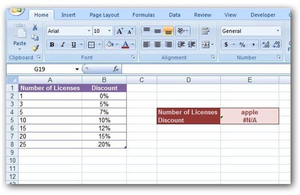
As mentioned when we were discussing the limitations of the LOOKUP function in a previous article in this series, an error message of the form #N/A will be returned if the lookup value of the function can’t be determined. For example, if we return to the function that we created in Part 1 of this series and entered the value “apple” for Number of Licenses (yes, things like this really do happen in the real world), we would see the following in our spreadsheet. (Click any image for a larger view.)
Changing Output of Error Messages
Even though we know that #N/A is an error message and it means that another value has to be entered for the function to calculate properly, others using the spreadsheet may not understand this message. Plus, this error message is just plain ugly. So, it’s worth the little extra effort to reformulate the LOOKUP function in order to give it a more customized error message that actually makes sense. We can do this by combining the LOOKUP function with the IFERROR function. (For more general information on this function, see Microsoft Excel’s IFERROR Function .)
Here, we would like to create a function that displays the value of the LOOKUP function if it exists or, otherwise, displays the message, “Please enter another value.” The standard format for the IFERROR function is
=IFERROR(standard function, message)
where the standard function, in this case, is our LOOKUP function and the message is the text or value that you would like to have displayed if the LOOKUP function cannot be calculated for some reason.
Taking the LOOKUP function we created in Part 1 of this series and combining it with the message above, we would obtain the following new function.
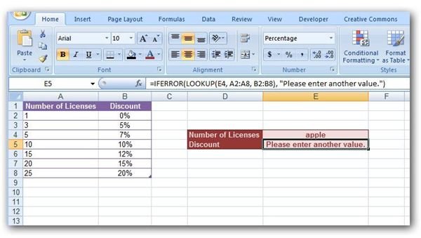
=IFERROR(LOOKUP(E4, A2:A8, B2:B8), “Please enter another value.”)
The screenshot below shows how this would appear in the Excel spreadsheet.
Note: You only need quotation marks in the message part of the IFERROR function if the message contains text. If you would prefer to replace the standard error message with a numerical value, such as 0, you can leave off the quotation marks.
Continue on to Part 3 of this series to learn about more specialized forms of the LOOKUP function, HLOOKUP and VLOOKUP. Also, be sure to browse through the rest of Bright Hub’s Microsoft Excel user guides to find other tips and tricks, including how to use Excel’s frequency function and detailed instructions for creating charts and graphs .
This post is part of the series: Microsoft Excel Lookup Functions
This series describes the construction and use of Microsoft Excel’s three basic lookup functions: LOOKUP, VLOOKUP, and HLOOKUP.


