The VLOOKUP and HLOOKUP functions in Microsoft Excel are powerful tools that can be used to query a lookup table, but many get confused when it comes to actually constructing formulas containing these functions. In this article, we’ll explain how to do this and give concrete examples.
Better Lookup Functions
While Excel’s LOOKUP function works well in very simple tables, it does have its limitations, as we discussed in Part 1 of this series. In most cases, it is better to use the HLOOKUP or VLOOKUP functions. These two functions are basically identical – the only real difference is that VLOOKUP is used when your data is arranged in columns and HLOOKUP when your data is arranged in rows.
Since HLOOKUP and VLOOKUP are so similar, we’ll concentrate on how to use VLOOKUP for now, since it is the most common. At the end of the tutorial, we’ll show how similar results can be obtained with HLOOKUP.
Walking Through Some Examples
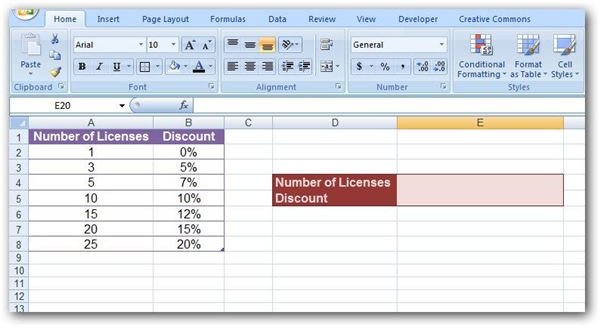
For this example, we’ll return to the table we used in Part 1 of this series. (Click any image for a larger view.)
Just as in Part 1, we want to construct a function that will return the applicable discount for a customer based on the number of software licenses that are purchased. The general syntax for the VLOOKUP function is
=VLOOKUP(lookup_value, table_array, col_index_num, range_lookup)
where each of the arguments of the function have the following meaning.
-
lookup_value – The value that you are looking up in the table.
-
table_array – The range of cells in which the data of the lookup table is stored.
Advertisement -
col_index_num – The number of the column in the table that contains the data that is to be returned by the VLOOKUP function.
-
range_lookup – This is an optional value that only has two possible states: True or False. If the value is set to False, the VLOOKUP function will only look for exact matches to the lookup_value in the table_array. If the value is set to True, the VLOOKUP function will try to return the best match in the same manner that the basic LOOKUP function does. That is, if an exact match isn’t found, it will return the result associated with the largest value that is smaller than the lookup_value. There are a couple of additional things to note about the range_lookup.
Advertisement
Note: If no value is specified for the range_lookup, it will default to True. If the value of the range_lookup is True, then the first column of the table_array needs to be sorted in ascending order to ensure that the VLOOKUP function works properly.
Now, let’s see what these arguments mean in terms of our example.
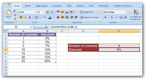
Referring back to our table in the screenshot above, we want to look up whatever value is entered for Number of Licenses in cell E4. So, this would be our lookup_value. The data in our table resides in columns A and B and in row 2 through row 8. This gives us a table_array of A2:B8. We want the VLOOKUP function to return the appropriate Discount which is found in the second column of the table, making our col_index_num equal to 2. In this example, we want more than just an exact match returned, so we’ll let the range_lookup retain its default value of True and not enter anything for this argument. Thus, our resulting function becomes:
=VLOOKUP(E4, A2:B8, 2)
A screenshot of how this would appear is shown below.
Note that this function can also be modified to display a customized error message whenever invalid data is entered into the Number of Licenses field. For more information on how to make these changes to the function, see Part 2 of this series.
Corresponding HLOOKUP Example
The construction of an HLOOKUP function is identical to that of its VLOOKUP counterpart, except that column values are replaced by row values. As an example, we’ll look at the same table of information that we have been using, but this time we’ll view it in a row format.
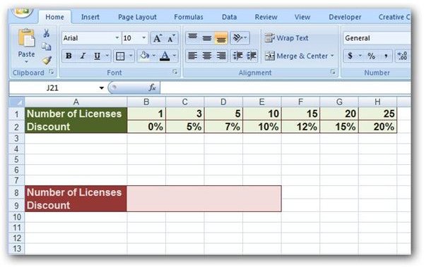
The general syntax for the HLOOKUP function is
=HLOOKUP(lookup_value, table_array, row_index_num, range_lookup)
where the arguments of the function have the same definition as those in the VLOOKUP function. The only difference here is col_index_num is replaced by row_index_num. Like its companion, row_index_num refers to the row number of the table that contains the information to be returned by the function.
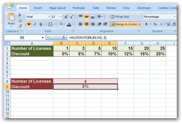
The HLOOKUP function that produces the same results in this table as the VLOOKUP function in the previous example is as follows:
=HLOOKUP(B8, B1:H2, 2)
Below is a screenshot of how this function would appear in the Excel spreadsheet.
References
- All screenshots taken by author.
- Microsoft Excel Official Site, http://office.microsoft.com/en-us/excel-help/
This post is part of the series: Microsoft Excel Lookup Functions
This series describes the construction and use of Microsoft Excel’s three basic lookup functions: LOOKUP, VLOOKUP, and HLOOKUP.


