In this Microsoft Excel tutorial, we’ll take a look at the construction of a basic LOOKUP function and how to use it to locate information in a table.
Basics on Lookup Functions
In Microsoft Excel, lookup functions are used to find a value that is associated with another entry in a table. For example, if we have a table containing a list of countries and their respective populations, we can use a lookup formula to find the current population of Denmark (or any other country in the list). These types of functions are particularly useful when dealing with data that is continuously being updated or modified.
There are many types of lookup functions in Excel, but in this series, we’ll concentrate on the three basic ones – LOOKUP, VLOOKUP, and HLOOKUP – and explain how they differ. We’ll begin with the LOOKUP function.
The LOOKUP Function
The most general lookup function, aptly called LOOKUP, will search a single row or column for a lookup value and return a result from another specified row or column.
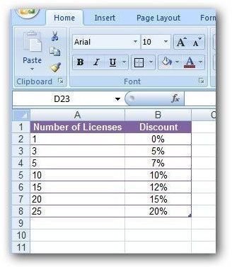
As an example, suppose that we have a table that contains information on the discount available for buying multiple licenses of a particular software product. (Click any image for a larger view.)
In this case, we’d like to be able to construct a function where customers can enter the number of licenses they wish to purchase and be told what discount would apply.
A LOOKUP function can be created using the syntax
=LOOKUP(lookup_value, lookup_vector, result_vector)
where lookup_value refers to the value that you want to find in the table, the lookup_vector designates the row or column in which you want to look for the value and the result_vector is the row or column containing the information that you want to “look up” for the value.
Before we go any further, it’s important to note some of the limitations of the LOOKUP function.
-
In order for the LOOKUP function to work properly, the values in the lookup_vector must be sorted and arranged in ascending order.
Advertisement -
If the function can’t find the exact lookup_value in the lookup_vector, it will use the largest value in the lookup_vector that is smaller than the lookup_value. For instance, if the values in the lookup_vector are 1, 5, 10, 20, and 30, and the lookup_value is 9, the LOOKUP function will return the result associated with the value of 5.
-
If all of the values in the lookup_vector are greater than the lookup_value or if the lookup_value doesn’t make sense in respect to the data in your table, the LOOKUP function will not be able to return a result, and an error message will be displayed.
Advertisement
How to Use the LOOKUP Function
Now, let’s return to our example and show how to construct a LOOKUP function that will give the applicable discount for purchasing a specified number of software licenses.
First, we’ll add a separate smaller table where customers can enter the number of licenses they wish to purchase.
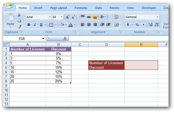
Note that in this example, the number of licenses will be entered in cell E4. This cell will be our lookup_value. We will be searching for this value in the column titled Number of Licenses, which contains values in cells A2 through A8. So, our lookup_vector will be A2:A8. We will want to return the corresponding percentage found in the Discount column, which contains values in cells B2 through B8. This will give us a result_vector of B2:B8. Putting these three items together, our LOOKUP function becomes:
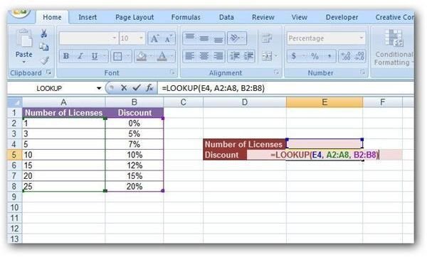
=LOOKUP(E4, A2:A8, B2:B8)
The screenshot below shows how this would be entered into the appropriate cell in Excel.
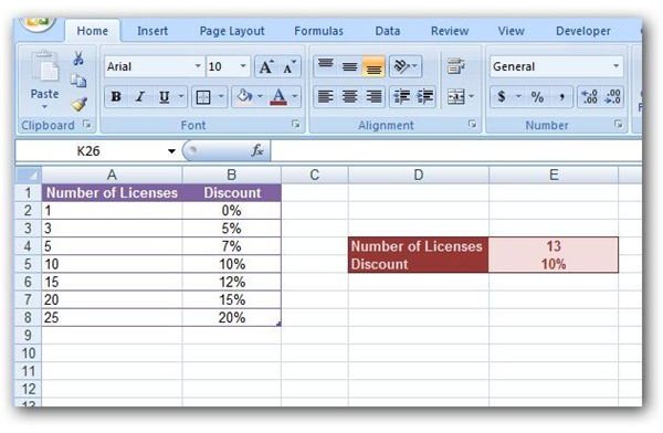
With this function in place, you can test it by entering a value for the Number of Licenses in cell E4.
We’ll look at more robust forms of lookup functions in Part 3 of this series, but first we’ll show how these tools can be combined with the IFERROR function to make error messages more meaningful. Continue on to Part 2 of this series to find out more.
This post is part of the series: Microsoft Excel Lookup Functions
This series describes the construction and use of Microsoft Excel’s three basic lookup functions: LOOKUP, VLOOKUP, and HLOOKUP.


