This Microsoft Excel function tutorial concentrates on the syntax and basic usage of the INDEX function. Read on to find out more.
Overview of the INDEX Function
Like the LOOKUP and MATCH functions, the INDEX function is another tool used to find information in an Excel list or table. One nice thing about the INDEX function is that its construction is a lot simpler than other lookup and reference formulas. This simplicity does mean that the INDEX function isn’t as robust as some of its counterparts, but it is still a good choice for the times when it does apply.
The Syntax of the INDEX Function
The basic syntax of the INDEX function is
INDEX(array, row_num, col_num)
where the arguments have the following definitions.
-
array – The array is the range of cells containing the table data that you want to query.
-
row_num – This value denotes the number of the row in the array that contains the information you want returned by the INDEX function.
Advertisement -
col_num – The col_num argument gives the number of the column from the array that contains the information you want returned by the INDEX function.
How to Use the INDEX Function
To illustrate the usage of the INDEX function, we’ll take the same example we used when explaining the OFFSET function in a previous tutorial. (Click any image for a larger view.)
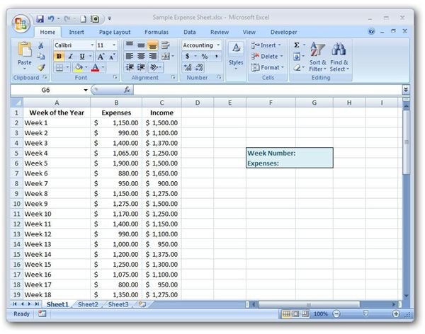
In this example, we have a table listing weekly expense and income reports. We would like to construct a function in which a user can enter a week number, and the expenses paid out during that week will be returned.
The data for the table is contained in columns A through C and in rows 2 through 53. So, our array for this example would be A2:C53.
Note, in this case, that the first row of the table is actually row 2 on the Excel spreadsheet. When determining what values should be used for the row_num and col_num, disregard the general spreadsheet rows and columns and use the relative positions in the table array.
We will be asking users to enter the week number in cell G5 of this spreadsheet. Note that the week number corresponds to the actual row number in the table array that contains the information for which we are looking. Thus, the row_num argument would be G5.
No matter which week is picked by the user, the expense information will always be found in the second column of the table. This gives us a col_num of 2.
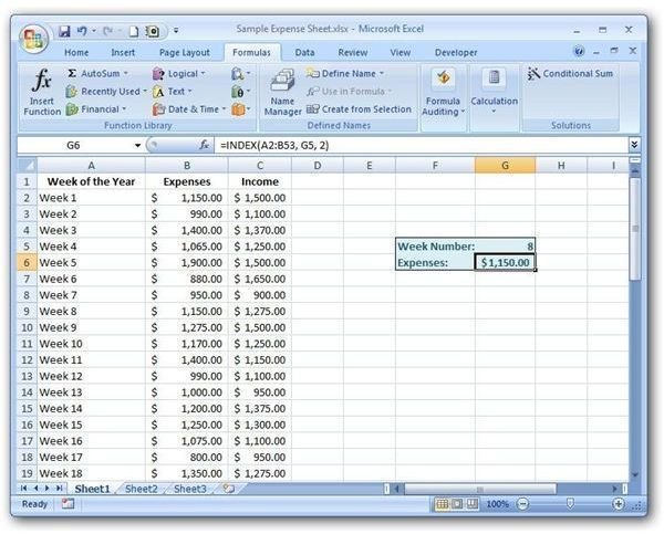
Putting all of this information together, our INDEX function becomes:
INDEX(A2:C53, G5, 2)
To see how this would appear in the Excel spreadsheet, take a look at the screenshot below.
It is possible to use other functions to get this same result. For a comparison, take a look at this tutorial covering the VLOOKUP function .


