The AND, NOT, and OR functions in Excel can be used to categorize data into smaller groups for further analysis. In this article, we’ll give examples of how each of these functions works.
Easy Way to Find Items on a Spreadsheet
Have you ever been presented with a spreadsheet containing hundreds, or even thousands, of rows of data and asked to find which items satisfy certain conditions? Sometimes, you can accomplish this task by using Excel’s sorting and filtering tools, but these weapons may not be so helpful if you want to perform additional analysis on the data without copying it to a new worksheet.
Another way to attack this type of problem is to use the AND, NOT, and OR logical functions found in the Formulas tab of Excel 2007. The beauty of using these functions is that they can be nested and combined with other functions to perform many different data operations. In later articles of this series, we’ll give some examples of how these functions can be combined with others, but at this time, we’ll restrict ourselves to just looking at their basic usage.
The AND Function
With the AND function, you can specify a number of conditions (up to 255) and receive a value of TRUE if all of the conditions are met. If even one of the specified conditions is not met, the AND function will return a value of FALSE.
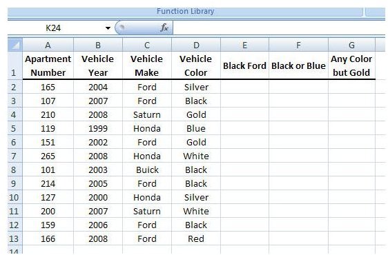
As an example, let’s suppose that we have a spreadsheet containing data for an apartment complex that lists the year, make, and color of each resident’s vehicle. The screenshot below shows how the information has been entered into the spreadsheet. (Click the image for a larger view.)
Using this data, we want to find out how many vehicles are black in color and made by Ford. We can use the following AND function to determine which vehicles meet both these conditions.
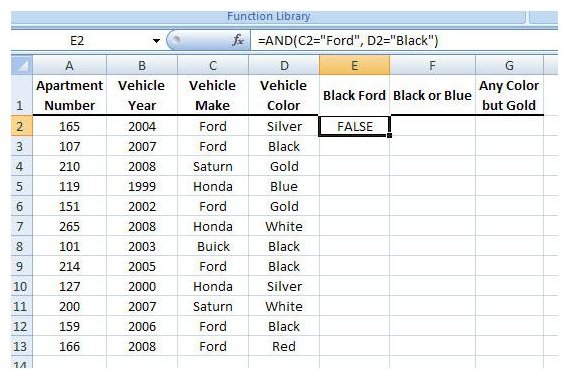
=AND(C2=”Ford”, D2=”Black”)
Entering this formula into the first empty cell of the Black Ford column yields the result shown below.
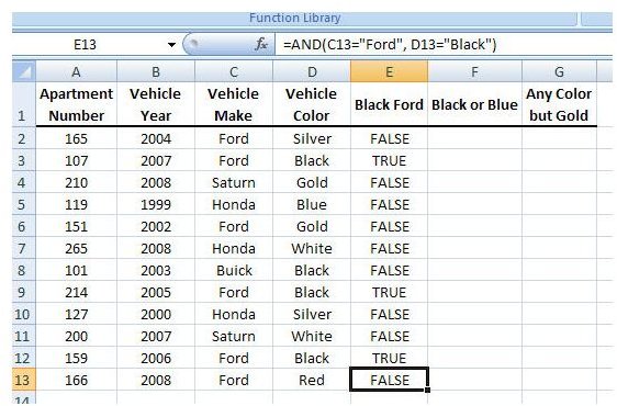
If we copy (or “fill down”) the function into the other cells of the column, we can see that the value of TRUE is returned for each row in which the Vehicle Color is black and the Vehicle Make is Ford. All other rows return a value of FALSE.
The OR Function
The OR function in Excel is very similar to the AND function, except that it will return a value of TRUE whenever at least one of the conditions of the functions is met. The only time that a FALSE value will be returned is when all the conditions are FALSE.
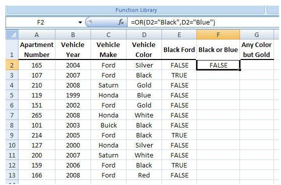
Using the same data as in our example above with the AND function, let us now suppose that we want to construct a function that will separate the vehicles that are blue or black from the rest in the list. To do this, we can use the following function.
=OR(D2=”Black”, D2=”Blue”)
This will appear in the spreadsheet as shown in the screenshot below.
After copying and pasting the function into the rest of the cells in the column, we obtain the following results.
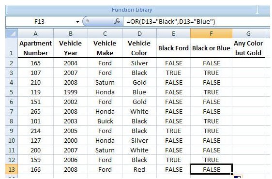
For each instance when the color of the vehicle is either black or blue, the value TRUE is returned. Otherwise, FALSE is returned.
The NOT Function
In some cases, we are more interested in determining when a certain condition isn’t met than when it is. For those times, it’s usually easier to invoke the NOT function.
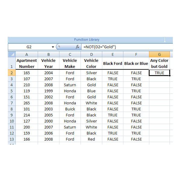
Using our example containing vehicle information, let’s develop a function that will select all vehicles with a color other than gold. We can use the following function.
=NOT(D2=”Gold”)
In our data list, this would appear as follows.
When we copy and paste the function into the other cells of the Any Color but Gold column, we obtain the results shown in the screenshot below.
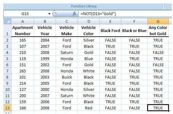
In this case, a value of FALSE is returned whenever the Vehicle Color is gold, and the value TRUE is returned everywhere else.
Applying Conditional Formatting
If we really want the cases when any of these functions evaluate to TRUE to stand out, we can apply a conditional formatting rule to the cells in the last three columns of our worksheet. To learn more about conditional formatting, check out the series Microsoft Excel 2007: Conditional Formatting . Even using a very basic rule here can make the TRUE values much easier to spot.
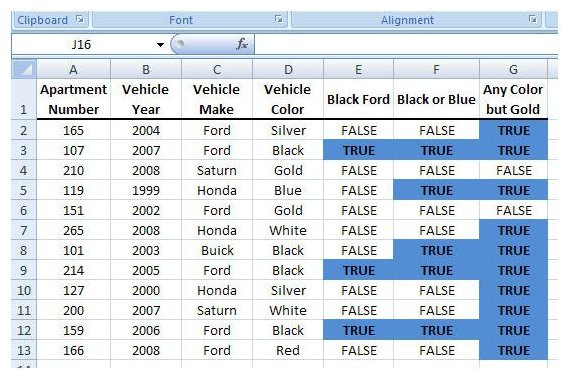
We could get a bit fancier here, but we’ll leave those instructions for the Conditional Formatting series. As mentioned in the opening section of this article, we will be looking at more advanced ways to combine logical functions in later segments of this series. Some of these methods provide a much nicer representation for data analysis so stay tuned!
This post is part of the series: How to Use Logical Functions in Microsoft Excel 2007
The logical functions of Microsoft Excel 2007 are extremely powerful tools that be used for many applications. This group of articles takes a look at individual logical functions available in Excel and describes how they can be used to save you time and improve your project analysis.


