How to Add a Background to a Spreadsheet and Simulate Watermarks in Microsoft Excel 2007
Watermarks and Spreadsheet Backgrounds
Although Word 2007 has a special tool that allows you to insert a watermark, there is no similar command in Excel 2007. However, it’s still possible to simulate a watermark on an Excel spreadsheet in several ways, one of which is by adding a background to the sheet.
How to Add a Background to an Excel Spreadsheet
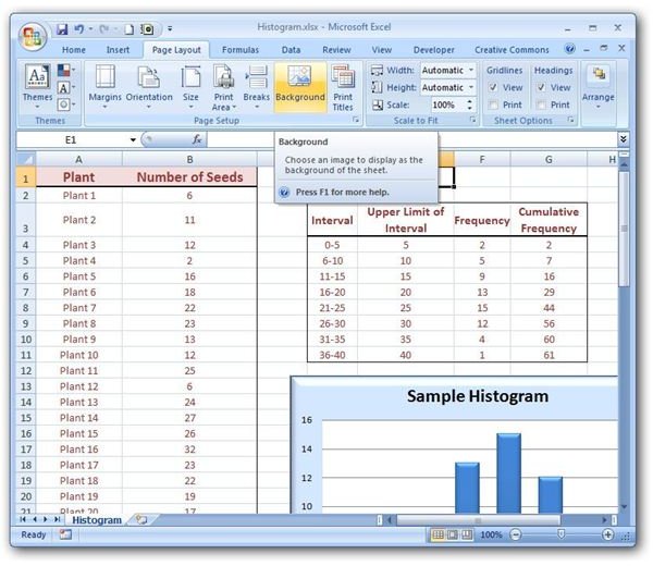
From the Page Layout tab on the Excel ribbon, select Background. (Click any image for a larger view.)
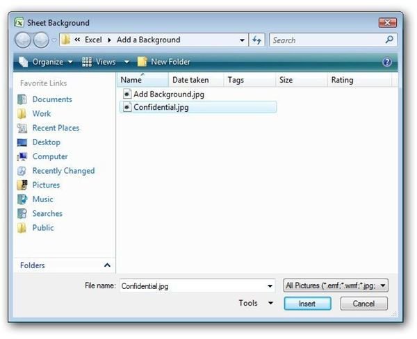
Navigate to the directory that contains the image file you want to use for the background, select the file, and click the Insert button.
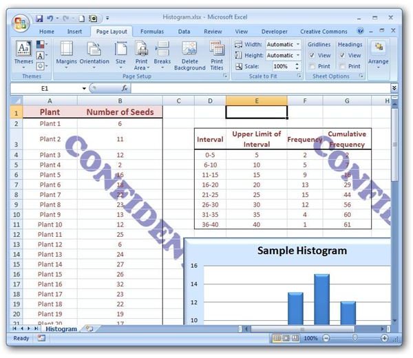
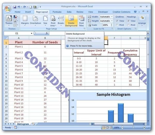
The image chosen will be tiled across the background of the spreadsheet as shown in the screenshot below.
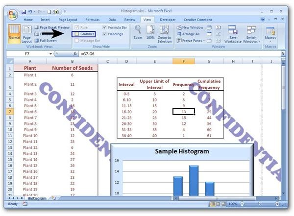
To improve the appearance of a spreadsheet with a background added, you may want to also remove the gridlines from that sheet. To do this, go to the View tab on the Excel ribbon and uncheck the box next to Gridlines.
Note that once you apply the background, you can’t make any adjustments to its size or appearance in Excel. So, if you’re not happy with how the background looks, you’ll need to remove it, edit the image in another application, and then add that modified image again.
How to Remove a Background
Removing a background from an Excel spreadsheet can be done with one click. Once a background has been added to a sheet, the text on the Background button on the Page Layout tab changes to read Delete Background. Click this button and the background will be removed.
More Tips for Improving the Appearance of a Background Image
If you have applied a fill color to any cell of your spreadsheet, that effect will obscure the background image. In order to make the entire image visible, change the fill color of any cells that are impeding the view to No Fill.
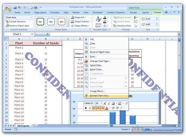
Charts, graphs, and other inserted objects will also block the view of the background image. However, for many of these items, you can adjust the transparency of the object to make the background viewable. For example, to adjust the transparency of a chart, right-click on the object and select Format Chart Area.
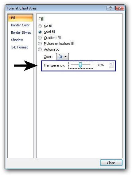
In the Format Chart Area window that appears on your screen, select Fill from the list of categories in the left panel of the window. Then, adjust the Transparency slider as much as needed. As you experiment with these settings, you’ll be able to see a preview in the Excel spreadsheet of how your proposed settings would appear. Click the Close button to apply the changes.
Other types of inserted objects can be modified in a similar manner.
For more tips and tricks, browse through Bright Hub’s library of Microsoft Excel user guides. These selections include design advice for charts and graphs, tips on how to record a macro, instructions for how to insert and remove Excel hyperlinks, and more. New articles are added to the collection on a regular basis, so remember to check back often!