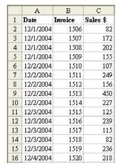
Problem: Your company offers a bonus pool on any day where the total sales exceed $1,000. You have invoice data by date, as shown in Fig. 1303. You would like to highlight all records for the days that meet $1,000 in sales.
Strategy: You can use conditional formatting to perform a complex task such as this. But first, before getting into conditional formatting, you should develop the formula that you will need.
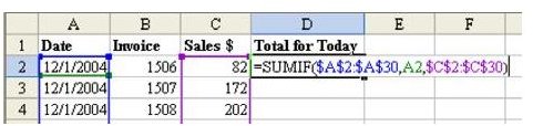
- The first task is to add a column that will total all sales for this day. As shown in Fig. 1304, the SUMIF function can do this. There are three arguments in the SUMIF function: =SUMIF($A$2:$A$30,A2,$C$2:$C$ 30).
This function tells Excel to examine each cell in A2:A30. If the cell value is equal to cell A2, then it adds up the corresponding cell from C2:C30.
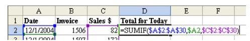
There are a lot of dollar signs in the formula. As you copy the formula down in your temporary column D, you want the ranges in the first and third parameter to be frozen. In our temporary formula in column D, there is no reason to freeze the A2 in the second parameter. However, in the conditional format dialog, this formula will be applied to cells in A, B, and C, so it is important to freeze the second parameter to column A.
-
In this case, you should edit the formula and add a $ before A2, as shown in Fig. 1305.
Advertisement -
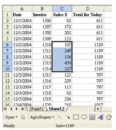
Enter the formula in D2. Double-click the Fill handle to copy the formula down. In Fig. 1306, you can see that every row contains the total sales for that day.
-
As a reasonableness test, highlight the sales for the December 2. The status bar at the bottom of the Excel window confirms that the total of these cells is $1,189.
Advertisement -
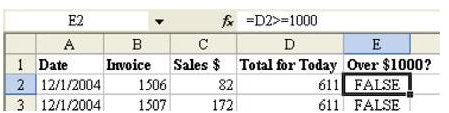
The formula for conditional formats requires a formula that evaluates to either TRUE or FALSE. Add a new formula in column E. As shown in Fig. 1307, the formula in E2 is =D2>=1000.
-
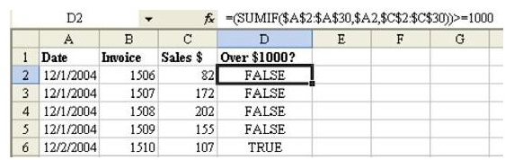
You can combine these two formulas into a single formula, as shown in Fig. 1308.
Advertisement
You now want to set up the conditional format. Follow these steps.
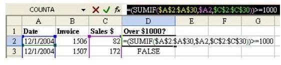
- It is easiest if you copy the formula that is working. Go to cell D2. Hit the F2 key to put the formula in Edit mode. In the formula bar, drag to highlight the entire formula, as shown in Fig. 1309.
-
Hit Ctrl+C to copy the formula from the formula bar. Copying from the formula bar allows the text of the formula to stay on the clipboard after you hit the Esc key.
Advertisement -
Hit the Esc key to exit Edit mode.
-
Select cells A2:C30. From the menu, select Format – Conditional Format.
Advertisement
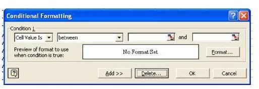
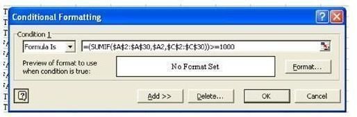
The Conditional Format dialog initially displays a format suitable for specifying that a cell contains a value between two other values, as shown in Fig. 1310. This is the easier version of conditional formatting, but it is the less powerful.
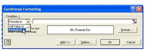
- To access the more powerful version, use the dropdown to change “Cell Value Is” to “Formula Is”, as shown in Fig. 1311.
-
Click in the formula box, and hit Ctrl+V to paste the formula from the formula bar, as shown in Fig. 1312.
Advertisement -
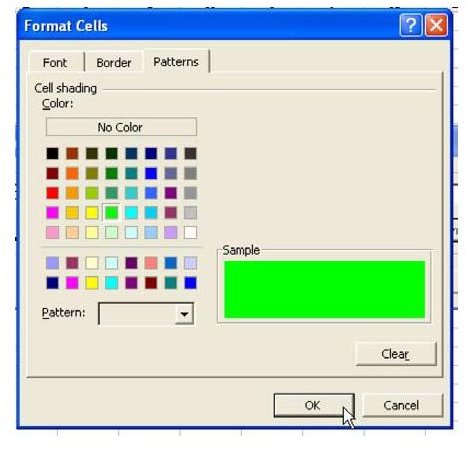
Next, you have to set up a unique format that should be used if the condition is True. Choose the Format… button. As shown in Fig. 1313, you will be given a dialog where you can customize the Font, Border, or Patterns.
-
Choose the Patterns tab. Select a green color and choose OK.
Advertisement -
Choose OK to close the Conditional Format dialog.
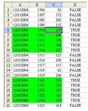
If everything worked OK, you will see that all of the rows for the second, fourth, and sixth are highlighted in green, as shown in Fig. 1314.
You can now safely delete your temporary formula in column D.
Summary: By changing the Conditional Formatting dialog from Cell Value Is to Formula Is, you can create amazingly powerful formulas to highlight entire rows if some condition is True.
Commands Discussed: Data – Conditional Format
Functions Discussed: =SUMIF()
Images