This article features a sample of an accounts receivable aging report in Excel format, as a useful tool for expediting report preparations. Readers will find the template available at Bright Hub’s Media Gallery; instructions to modify the formula and replace the data are furnished in this article
Using an Accounts Receivable Aging Report: Excel
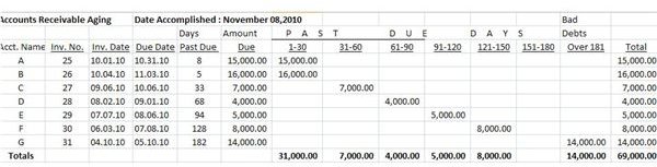
Using an accounts receivable (AR) aging report in Excel format expedites the process of report preparation, since the cells for the DATE inputs are formatted with formula for functions. The objective is to determine, at an instance, the length of time each receivable has remained unpaid beyond its maturity date at any given date of an AR aging report.
A sample of an Excel Accounts Receivable Aging Report Excel Template can be downloaded at Bright Hub’s Media Gallery. Readers who are interested in using it as their template can modify the report by replacing the information therein. Find instructions and explanations in the section below on how to fill each cell; you may need to customize the cell formula according to your own credit terms.
Instructions and Explanations on How to Replace Inputs
The Date (A1) – This will serve as the reference point for the Past Due Days column. Modify the date in cell B1 by using the numeric mm/dd/yyyy format: 11/07/2010
Account Number Column (A) – Simply index this column with the company’s control number for past due accounts receivable. This is important for maintaining the traceability of data against other accounting records, i.e. accounting entry tickets or vouchers, sales invoices, et al.
Invoice Number Column (B) – Input your invoice number — it is not necessary for the numbers to appear in proper numerical sequence, since not all accounts receivable are being aged. Nevertheless, this information is important to allow for audit trace-back purposes.
The Due Date Column (C) – The information in this column will be used to format the cells in column D to generate the maturity dates for each account.
The Maturity or Due Date Column (D) -- In our example, the due date is automatically generated using the 30-day credit term; hence this cell will reflect the account’s maturity date, accordingly.
To modify the template according to your own credit terms, refer to the formula bar and then change the term that is added to the cell reference number. To illustrate, let’s say you’re moving from cell D4 to D5 but the term for this account is 15 days instead of 30: Modify C5+30 appearing on the formula bar to C5+15. The cell will automatically return with the corresponding maturity date for a 15-day credit term and will likewise automatically input the number of Past Due Days in column E accordingly.
The Past Due Days Column (E) – The input in this cell is automatically generated by the functions of the cells in column D. As mentioned earlier, the D column automatically computes the number of days the account has been past due, based on the corresponding due dates generated under the Due Date column (D) and as of the report date you indicated in column B.
Amount Due – Place the corresponding principal amount or balance of the receivable under this column.
Past Due Days Column (1-30/ 31-60/ 61-90/ 91-120/ 151-180/ and Over 181) – Extend the amount due under the applicable column according to the number of Past Due Days generated under column E.
Totals – Totals can be generated through the auto sum function, by highlighting all cells from G4 to G12 extending through N4 to N12.
Once you have customized the formula values for the D columns, you can simply change the report date every time a new report is prepared and the number of past due days will be readily available.
To further appreciate the significance and uses of the accounts receivable aging report in Excel formats, it may interest the readers to view another Bright Hub article entitled: Accounts Receivable Aging: Understanding its Mechanics .
Reference Materials and Image Credit Section:
Reference and Image Credit:
- Author cscantoria’s personal files for Accounts Receivable Audit Procedures and Techniques