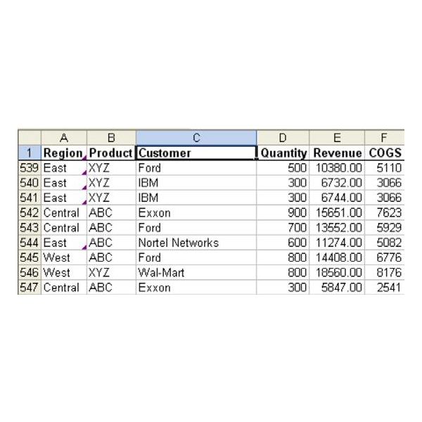
Problem: You need to include a calculation in the pivot table that is not in your underlying data. Your data includes Quantity Sold, Revenue, and Cost, as shown in Fig. 980. You would like to report Gross Profit and Average Price.
Strategy:
You can add a calculated field to a pivot table. Follow these steps.
-
Build a pivot table.
Advertisement -
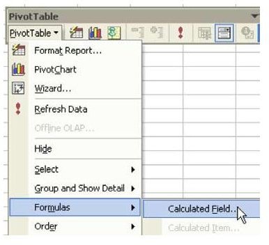
From the PivotTable toolbar, select PivotTable – Formula – Calculated Field, as shown in Fig. 981.
-
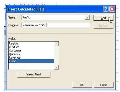
Type a name for the field, in this case, Profit. Enter the calculation =
Advertisement
R e v e n u e – COGS. Choose the Add button, as shown in Fig. 982.
-
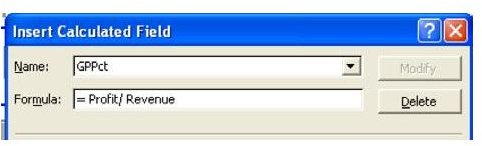
Here is the formula for Gross Profit Percent. See Fig. 983.
Advertisement -
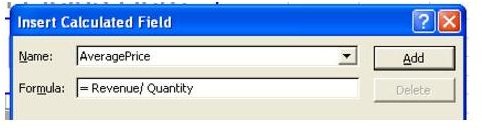
The formula for Average Price is shown in Fig. 984.
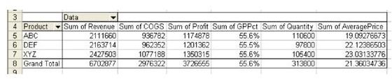
The resulting pivot table includes all of the fields, as shown in Fig. 985.
**
Gotcha:
The label Sum of GPPct is somewhat misleading, as is Sum of Average Price. In reality, Excel finds the sum of Revenue, finds the sum of Quantity, and then divides the values on the total line in order to get the average price. This makes calculated fields fine for any calculations that follow the Associative law of mathematics. If you actually wanted to have Excel do all of the individual average prices and then sum them up, it would be impossible in a pivot table.
Summary:
Calculated Fields add a new measure that can be reported in the Data area of a PivotTable for all Measures.
Commands Discussed:
PivotTable – Formula – Calculated Field
**
Images