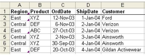
Problem: You work in a manufacturing plant, scheduling orders and material. You always appreciate it when the sales force gets orders a few months in advance so that you have enough time to get material into the plant without having to pay exorbitant prices on the gray market. Your dataset has both an Order Date and a Ship Date, as shown in Fig. 930. You want to analyze what percentage of the revenue comes in two months before the order has to ship.
Strategy:
****
You would like to build a pivot table report with OrdDate in the Column area, ShipDate in the Row area, and Revenue in the Data area. However, both of the date fields have more than 255 points, so you cannot initially produce a report with dates going across the columns.
-
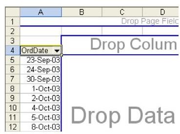
Initially, drag the OrdDate field to the Row area, as shown in Fig. 931.
-
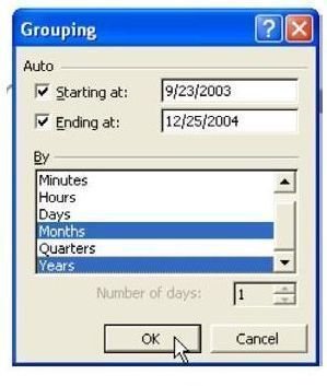
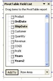
Right-click OrdDate. Choose Group and Show Detail – Group. Choose to Group by Months and Years, as shown in Fig. 932.
Advertisement -
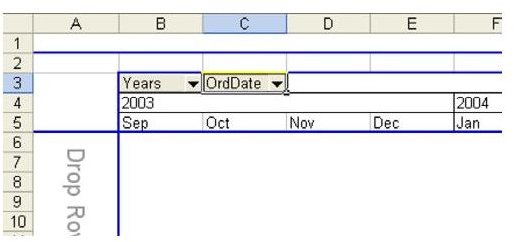
Now that the OrdDate field contains only 16 data points, you can drag Years and OrdDate to the Column area as shown in Fig. 933.
-
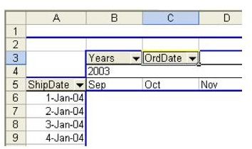
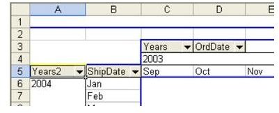
Next, drag the ShipDate field to the Row area, as shown in Fig. 934.
Advertisement
- Right-click ShipDate. Choose Group and Show Detail and then Group. Group by Months and Years, as shown in Fig. 935.
It is interesting that the OrdDate fields get a name of “Years”. When you group the Ship- Date field, the second field is called “Years2”, as shown in Fig. 936. There is really nothing in the PivotTable Field List to help you remember which Year goes with which date.
It might help to write a note in the worksheet to help you remember that you grouped ShipDate second and that the Years2 field is associated with ShipDate instead of Ord-Date.
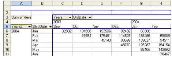
- Drag Revenue to the report, as shown in Fig. 937.
In Fig. 937, Cell G6 is an interesting number. It says that $60,368 of
the orders that shipped in January was also ordered in January. Your
manufacturing plant has to keep a lot of excess inventory on hand to be
able to react to orders that come in this late. Cell F6 shows that $92K of
orders for January was placed in December. This is still probably inside
the cumulative lead-time for most products.
**
Additional Information:
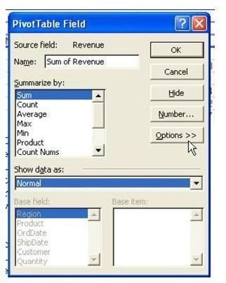
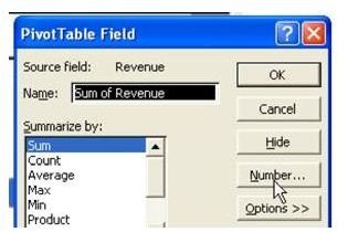
Double-click the Sum of Revenue button to display the Pivot- Table Field dialog. As shown in Fig. 938, choose the Options» button to unhide a powerful feature of Pivot Tables: Show Data As.
-
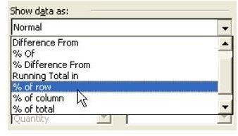
By default, the Data fields are shown as “Normal”. This means that Excel reports actual total revenue numbers in the report. There are many options available in the Show Data as: dropdown.
Advertisement -
In this case, choose Percentage (%) of Row, as shown in Fig. 939.
-
Before closing the PivotTable Field dialog, choose the button for Number…, as shown in Fig. 940.
Advertisement
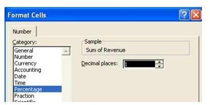
- Choose Percentage with one decimal place, as shown in Fig. 941. Choose OK to close the Format Cells dialog, then OK to close the PivotTable Field dialog.
Result:
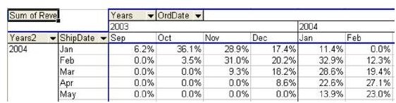
The pivot table shows that 11.4 percent of January 2004 shipments were ordered in January. See Fig. 942.
Summary:
This report required several techniques. Two different Date fields were grouped by month and year. You also had to double-click the Sum of Revenue field to set the number format and to change the reporting from Normal to Percentage of Row. This type of report will be very useful to all schedulers in manufacturing plants.
Commands Discussed:
Data – PivotTable – Show Data As; Data – PivotTable – Group and Show Detail
**
****
Images