How to Use Variations of the AVERAGE Function in Excel

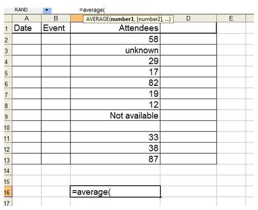
AVERAGE is a statistical function used to find the “arithmetic mean” (which is a fancy term for the average) of the values in the cells you select and apply it to. Using the AVERAGE function is pretty simple and straightforward. Start by clicking the cell in which you want the average to appear. Click inside the Formula Bar and type in =average( making sure to include the parentheses. You will see a screen tip that says AVERAGE(number1,[number2],…).This is your cue to select the numbers of which you want an average.

So Many Ways to Average

Drag your mouse down the column or across the row containing the numbers you want to use, or press and hold the Ctrl key to select incongruous cells. Once you have made your selection, press enter.

Another variation of Excel’s AVERAGE function is DAVERAGE. This function determines the average of cells in a database table that meet specific criteria. The syntax of the DAVERAGE feature is =DAVERAGE( table , column , criteria).

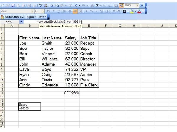
For our example, we have created a table in cells B3:E12 and we want to know the average salary for all of the employees listed in the database table. We do not want to include any salaries below 20,000. So we also entered Salary in cell B17 and >20000 in cell B18.

Start by selecting the cell in which you want the average salary to appear. Go to the Formula Bar and enter =****DAVERAGE( B3:E12 , “Salary” , B17:B18 ). Press the Enter key and you will have the averages of all salaries in the table above 20,000.

Excel’s AVERAGEA variation is quite similar to the original AVERAGE function. The primary difference is that if you have a cell selection containing text or blank cells and you use the AVERAGE function, those cells will be ignored. If you select the same range of cells and apply the AVERAGEA function, those cells will be included with a zero value. In our example, cells C2:C13 contains the number of attendees for different events. Some of the cells are blank, though, and others include text stating the data is not available. To find out the average, including the events that have no information, select the cell which you want to contain the average, go to the Function Bar and enter =averagea( again, including the parentheses.

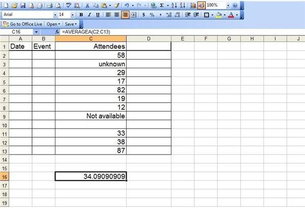
Select cells C2:C13 and press the Enter key. If you do not want the extensive decimals listed, select the cell, right click and choose Format Cells. On the Number tab, select Number in the Category list. Choose the number of decimal places you want, if any.

To learn even more about Excel’s extensive list of functions, check out the BrightHub article, Understanding Microsoft Excel Functions.