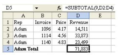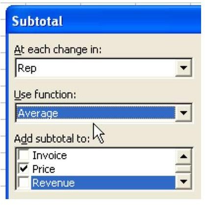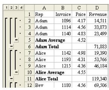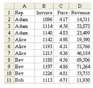
Problem: In the dataset in Fig. 753, you want to create a subtotal of revenue. It does not make sense to subtotal the unit prices in column C. It might make sense to create an average price for each rep.
When you add subtotals to a dataset, the function used is the SUBTOTAL function. As shown in Fig. 754, the formula automatically added to cell D5 is =SUBTOTAL(9,D2:D4).
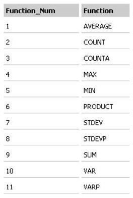
You can imagine that after creating the SUBTOTAL function, the team at Microsoft realized that they also needed SUBAVERAGE, SUBMIN, SUBMAX, and SUBCOUNT. Rather than create nine different functions, they created one function. The first parameter indicates whether Excel should average, sum, count, min, or max, etc. Fig. 757 shows the complete table of values.
Note: In Excel 2003, Microsoft added the 11 new function numbers. From 101 to 111, they do the same functions as 1 through 11, but ignore hidden rows.
If you attempt to add a Sum subtotal to revenue and then add an Average subtotal to Price, the subtotals appear on two lines, as shown in Fig. 758. This may not be what you want.
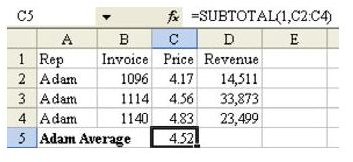
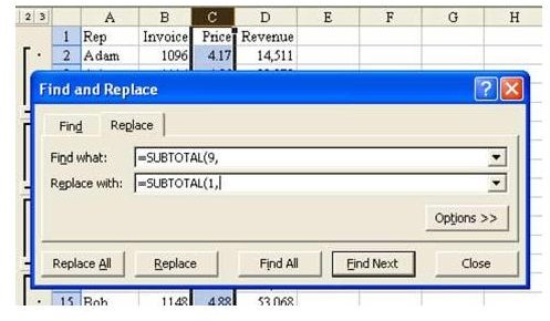
An alternate method is to add Sum subtotals to both columns. The intermediate result will not make sense for the Price column. Select column C and from the menu choose Edit – Replace.
As shown in Fig. 759, in the Find and Replace dialog, specify that you want to change every occurrence of =SUBTOTAL(9, to =SUBTOTAL(1,.
It is important that you only select column C before you replace, otherwise you will replace the formulas in the Revenue column as well.
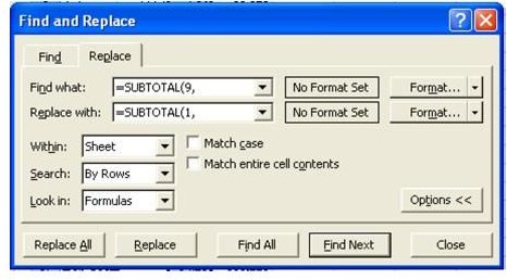
It is worth noting that the Find and Replace dialog remembers settings from the last time it was used in the current Excel session. There are settings in the Options» button that are right by default, but might have been changed if you did a Replace or a Find since you launched Excel. Choose the Options» button. Make sure that the Look In dropdown is set to Formulas. As shown in Fig. 760, make sure that the Match Entire Cell Contents checkbox is unchecked.
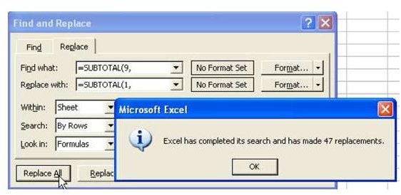
Choose the Replace All button. Excel will confirm how many cells have been changed. As shown in Fig. 761, a good reasonableness test is to check whether your company has 47 sales reps.
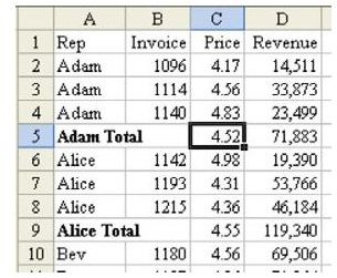
Result: As shown in Fig. 762, the revenue is totaled and the prices are averaged on the subtotal lines.
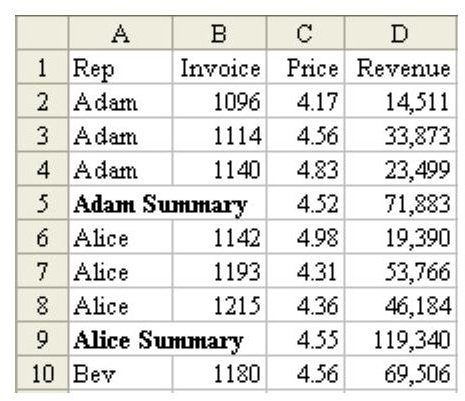
Additional Details: In Fig. 762, note that the subtotal lines declare “Adam Total”. This is technically incorrect. You could select column A and change every occurrence of “Total” to “Summary”, as shown in Fig. 763.
Gotcha: Be careful when using Edit – Replace. While it is unlikely that you have any sales reps with “SUBTOTAL” in their name, it is possible that you might have customers with “sum” in their name. Be sure to only select the relevant columns before doing the Find and Replace. To avoid inadvertently changing “Summervilles” to “Averagemervilles”, it helps to make sure that the text being changed is unique. You can usually do this by including the opening parenthesis in the original and changed text. Making sure to change “SUM(” to “AVERAGE(” is a simple but important step to prevent accidentally changing “summary” to “averagemary”.
Summary: Use Edit – Replace to change the SUBTOTAL function from a sum to an average. This allows you to have one summary line per rep, with different types of subtotals.
Images