In this article, I will explain everything you need to know about Microsoft Excel Formulas and Functions. After reading this tutorial, you will be well on your way to becoming a Excel Ninja.
Microsoft Excel Spreadsheet Formulas
In this tutorial, I will tell you everything you need to know about Microsoft Excel spreadsheet formulas.
Microsoft Excel is a wonderful tool used by professionals worldwide. It is the most popular spreadsheet application and is available on Windows and Mac OS X. The latest version of Microsoft Excel is Excel 2010.
Microsoft Excel also includes a programming component based on Visual Basic for Applications.
Excel also includes a wide range of spreadsheet formulas which you can use to automate your workflow and make it easier along with macros . After completing this tutorial, you will know everything there is to know about Excel formulas and functions.
You can use either direct values in Excel : values like numbers (1,2,3,4.5,12.10 etc) or strings (“BrightHub”, “Pathik”, “Awesome”).
You can also use cell values as variables. For example, to use the value in the first cell as a variable, use A1. For the cell in the first row and 5th column, use E1.
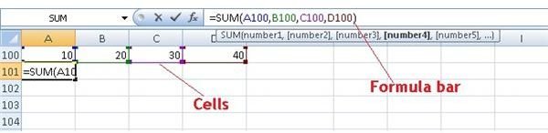
All Excel formulas and functions start with a “=” sign.
For example, =SUM(A1,B1) will give you the sum of the values in the cells A1 and B1. You can enter the formula syntax in the function bar on the top.
I will list all the basic in Microsoft Excel Spreadsheet Formulas and Functions.
Mathematical Formulas in Excel
SUM(value1, value2)
This returns the sum of the 2 values.
For example,
=SUM(1,2) returns 3
=SUM(A1, B1) returns the sum of the values stored in A1 and B1
PRODUCT(value1, value2)
This returns the product of the 2 values.
For example,
=PRODUCT(2,3) returns 6
=PRODUCT(A1, B1) returns the product of the values stored in A1 and B1
POWER(value1, value2)
This returns the value of value1 raised to the power of value 2.
For example,
=POWER(2,3) returns 8
=POWER(A1, B1) returns the value of value1 raised to value2.
RAND
This returns a random number between 0 and 1
=RAND() could return 0.53545 or 0.98273
ABS(value)
This returns the absolute positive value of the value or number entered.
For example,
=ABS(5) returns 5
=ABS(-10) returns 10
CEILING(value, significance)
This returns the value of the number entered rounded up to the nearest multiple of significance.
The significance is the unit you want to round it up to. CEILING always increases the absolute value of the number
For example,
=CEILING(5.4,1) returns 6
=CEILING(-10.2,-1) returns -11
FLOOR(value,significance)
This returns the value of the number entered rounded down to the nearest multiple of significance.
The significance is the unit you want to round it down to. FLOOR always decreases the absolute value of the number
=FLOOR(5.4,1) returns 5
=FLOOR(-10.2,-1) returns -10
GCD(value1, value2)
This returns the greatest common divisor (GCD) of the two numbers.
For example,
=GCD(20,15) returns 5
=GCD(A1,B1) returns the GCD of the values stored in A1 and B1
LCM(value1, value2)
This returns the least common multiple (LCM) of the two numbers.
For example,
=LCM(20,15) returns 60
=LCM(A1,B1) returns the LCM of the values stored in A1 and B1
LOG(value1, base)
This returns the log of the value to the base. If no base is specified, the default base is 10.
For example,
=LOG(10) returns 1
=LOG(10,2) returns 3.321928
Besides these, there are also the trigonometric formulas .
The most basic ones are
PI
This returns the value of the trigonometric constant Pi.
=PI() returns 3.141593
SIN(value1)
This returns the sine value of the variable specified in radians
=SIN(10) returns -0.54402
COS(value1)
This returns the cosine value of the variable specified in radians
=COS(10) returns -0.83907
TAN(value1)
This returns the tangent value of the variable specified in radians
=TAN(10) returns 0.648361
Text Functions in Excel
Text functions are the most widely used after math functions
CHAR (value1)
This returns the character corresponding to the given ASCII value
=CHAR(97) returns the result “a”
=CHAR(100) returns the result “d”
CODE (value1)
This returns the ASCII code for the character value
=CODE(“a”) returns the value 97
=CODE(“z”) returns the value 122
LOWER(string)
This returns the string in lowercase
=LOWER(“Brighthub is an awesome WEBSITE”) returns the string “brighthub is an awesome website”
UPPER(string)
This returns the string in uppercase
=UPPER(“Brighthub is an awesome WEBSITE”) returns the string “BRIGHTHUB IS AN AWESOME WEBSITE”
PROPER(string)
This returns the string in the proper case with all first characters capitalized.
=PROPER(“Brighthub is an awesome WEBSITE”) returns the string “Brighthub Is An Awesome Website”
CONCATENATE(string1, string2)
This concatenates the two strings specified and returns “string1 + string2”
=CONCATENATE(“Brighthub “, “Pat”) returns “Brighthub Pat”
=CONCATENATE(“Brighthub “, A1) returns “Brighthub (value in A1)”
LEN(string value)
This returns the length of the specified string.
=LEN(“Lalalalalala”) returns 12
SEARCH(character, string to be searched, starting position)
This returns the position of the specified character or string in the given string.
=SEARCH(“h”, “Brighthub”, 1) returns 5
These are the basic text functions in Microsoft Excel
Logical Functions in Excel
AND (condition1, condition2)
This function will return true only if both condition1 and condition2 are true, else it will return false
=AND(1<2,1<3) returns TRUE
=AND(1>2,1<3) returns FALSE
OR (condition1, condition2)
This function will return true even if any one condition is true, it will return false only if both are false else it will return false
=OR(1>2,1>3) returns FALSE
=OR(1>2,1<3) returns TRUE
NOT(statement)
This returns the opposite of the value returned by the statement
=NOT(TRUE) returns FALSE
=NOT(1<2) returns FALSE
IF(condition, truevalue, falsevalue)
The IF function returns truevalue if the condition is true and falsevalue if the condition is false.
=IF(1<2, “1 is less”, “2 is less”) returns “1 is less” as the condition is true, 1 is less than 2.
Statistical Formulas in Excel
MAX(value1, value2, value3)
This returns the maximum value from the list of values provided
=MAX(1,2,3,4) returns 4
MIN(value1, value2, value3)
This returns the minimum value from the list of values provided
=MIN(1,2,3,4) returns 1
AVERAGE(list of values)
This returns the average of the list of values specified
=AVERAGE(1,2,3,4,5) returns 3
MODE(list of values)
This returns the mode of the list of values specified
=MODE(1,1,3,4,5) returns 1
MEDIAN(list of values)
This returns the median of the list of values specified
=MEDIAN(1,2,3,4,5) returns 3
COUNT(list of values)
This returns the count of the total number of values present in the list
=COUNT(1,2,3,4,5,1,2,3,4,5) returns 10
Date and Time Formulas in Excel
This is the last major type of functions. It returns the date and time of the system which Excel is running on.
=NOW()
This returns the current time and date
=TODAY()
This returns today’s date
=DATE(year, month, date)
This returns the specified date in the correct format
=TIME(hour, minute, second)
This returns the specified time in the correct format.
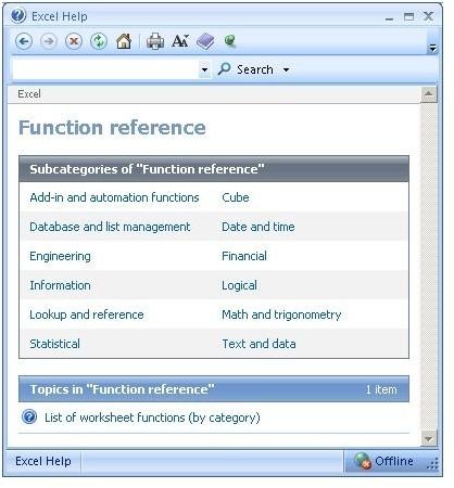
These are all the basic functions you will use in your Excel spreadsheets. There are many more functions which you can access directly from Microsoft Excel’s help. Just open up Microsoft Excel and press F1 to launch the Help window and search for the function you want.