In this Microsoft Excel tutorial, we’ll describe the MATCH function and how it can be used to determine the position of an item in a list or table.
The MATCH Function
The MATCH function is a special type of lookup function in Microsoft Excel that will search for a given entry in a table and return the relative row or column position of that value. There are many applications for this function, but one of the most common uses is to determine the rank of an item in a list.
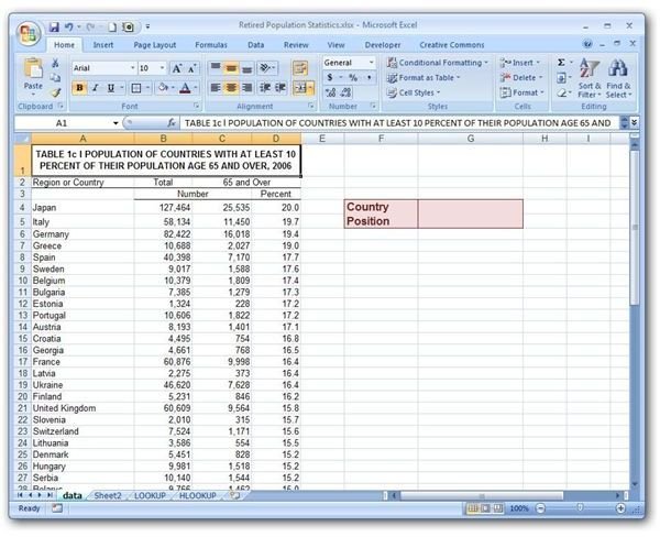
For example, the screenshot below shows a table listing countries with at least 10% of their total population consisting of people over the age of 65. The source data for this table can be found at the Federal Interagency Forum on Aging-Related Statistics .
(Click any image for a larger view.)
This table has been sorted and ordered based on percentage of population over the age of 65. We’d like to construct an example where the name of any country can be given and a MATCH function will return its ranking on this list.
Syntax of the MATCH Function
The basic syntax of the MATCH function in Excel is
MATCH(lookup_value, lookup_array, match_type)
where the arguments in the function have the following meanings.
-
lookup_value – The value to be looked up in the table.
-
lookup_array – The range of cells containing the table data.
Advertisement -
match_type – The match_type is an optional argument that can be set to one of three values: -1, 0, or 1. If the value is set to 0, the MATCH function will locate the first instance of the lookup_value in the lookup_array and return its position. If the value is set to -1, the MATCH function looks for the smallest value in the lookup_array that is greater than or equal to the lookup_value. For a match_type of 1, the MATCH function searches for the largest value in the lookup_array that is less than or equal to the lookup_value. If no match_type is specified, this value defaults to 1.
Note: Just as in the case with the LOOKUP function , MATCH functions with match_type 1 must be sorted in ascending order. Opposite of that, MATCH functions with match_type -1 must be sorted in descending order. However, if you choose 0 for your match_type, no sorting of the data is needed.
How to Use the MATCH Function
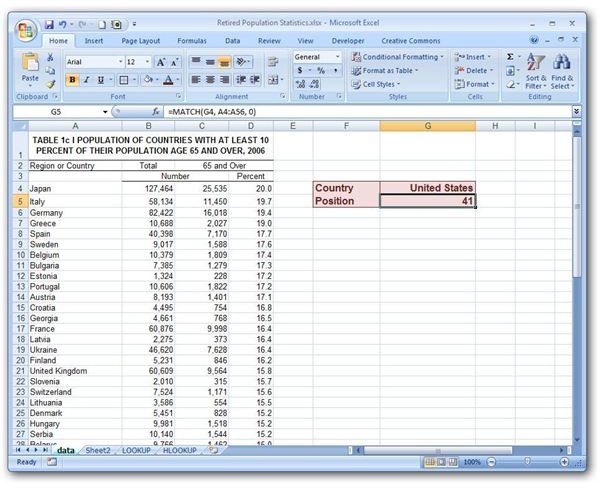
Going back to the table in our initial screenshot above, we want to define a MATCH function that will take a country’s name entered in cell G4 and return its ranking from the population list. Thus, our lookup_value is G4. Since the listing of countries is contained in cells A4 through A56, our lookup_array is A4:A56. Further, since we don’t want to sort this list of countries by name of the country (we want to keep it sorted by percent of population over the age of 65), we want to use a match_type of 0.
All of this would translate to the following MATCH function.
MATCH(G4, A4:56, 0)
The screenshot below shows how this function would appear in the Excel spreadsheet.
It’s important to note that when using a match_type of 0, an error message of #N/A will appear if no exact match is found for the lookup_value. To find out how to change this error message to something more meaningful, see the article Customizing the Error Value for a LOOKUP Function . Also, check out the other Excel function tutorials in Bright Hub’s collection, including how to use the FREQUENCY function and how to construct nested IF functions .


