Filtering is the process of temporarily removing some data from sight so that you can work with only the data you need. Read on to learn how to filter information in Excel 2007 to reduce the time you spend working with spreadsheets.
Spreadsheets are so common in business and home applications that they have become an indispensable tool for storing, retrieving, and manipulating data. However, many business and home users do not venture beyond the basic spreadsheet functions. One of the most powerful yet often overlooked functions in Excel 2007 is the filter command. Using filtering in Excel 2007, you can temporarily remove from sight information you don’t care about at the moment. With a click of the mouse, you can remove filtering and see all of your data again.
Suppose you have a column of data that contains similar items in each of the cells. With the filtering command, you can temporarily hide certain data so that you are not constantly searching up and down your columns for the information you need. Learn how to successfully use the filter functions in Excel 2007 and spend less time hunting for data in large Excel files.
How to Use the Filter Command in Excel 2007
Filtering data in Excel 2007 is not unlike sorting. However, rather than order data in a more convenient way, you can temporarily hide data so that you can speed up your work process. When you are done, you un-filter the data and continue working in your Excel 2007 spreadsheet normally.
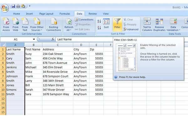
Suppose you have an address list in an Excel 2007 spreadsheet and you want to see only the addresses of people who have the last name “Smith.” To begin your filter, click on the column that contains the data you want to filter. Then, click on the DATA tab on the Excel 2007 Ribbon and click on the FILTER button (see Figure 1).
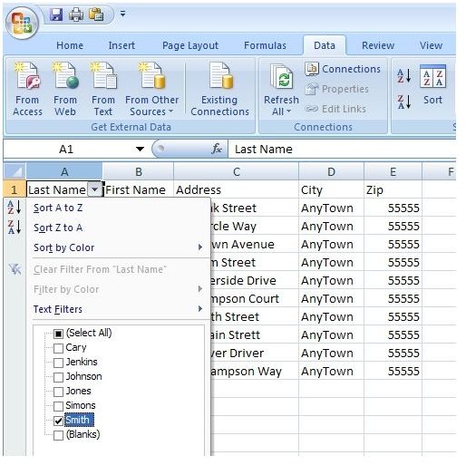
When you click on the FILTER button, an arrow appears at the top of the column that contains the data you want to filter (see Figure 2). Click the arrow and then click on the check mark next to the SELECT ALL option. This simply clears all of the checks next to each of the data points in that particular column. Now place a check mark next to the data points you want to filter. In this case, check the box next to the data labeled “Smith.”
Click OK and notice that the spreadsheet now only displays data where the LAST NAME column contains the text “Smith.” Notice also that the arrow next to the LAST NAME column shows a picture of a funnel and that there are now “missing” row numbers down the left side of the spreadsheet. These row numbers are now blue rather than the default black. This is to remind you that you are viewing filtered data, not all of the information contained in the spreadsheet.
To view all of the data in the spreadsheet again, click on the funnel icon at the top of the LAST NAME column and check SELECT ALL. Now you are seeing all of the data in the spreadsheet again.
To turn off the filtering permanently, click again on the FILTER command button on the DATA tab of the Excel 2007 Ribbon. Note that unless you click the FILTER button on the Ribbon after you are done filtering, Excel 2007 remains in filter mode. While in filter mode, you may not be able to use all of the functions in Excel. Some of the functions that would conflict with filtering are disabled. Therefore, be sure to click on the Filter command on the Ribbon when you are done filtering to make Excel fully functional again.
Conclusion
Filtering data in Excel 2007 allows you to view only the information you want to see at the moment. Filtering makes large spreadsheets more manageable and also reduces the time you spend looking for and manipulating data in your file. You can use filtering and then turn it off with just a few clicks of the mouse, making filtering a powerful yet strangely overlooked function in Excel 2007.


