Excel 2007’s SmartArt charts make it easy to create a hierarchal diagram, workflow process, or specialized table or list within a spreadsheet. In this tutorial, we’ll show how to insert and modify these useful charts.
Specialized Charts and Trees in Excel 2007
Mention Excel and charts in the same sentence, and many people envision the standard pie charts and histograms that present figures and percents. However, there is another type of chart feature in Excel that lets users create diagrams, tree structures, and other similar objects. This underestimated tool goes by the name of SmartArt.
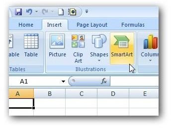
To access this feature, open the Insert tab on the Excel ribbon and click on SmartArt in the Illustrations category of the tab. The location of this button is shown in the screenshot below. (Click any image for a larger view.)
This will open a new window where you can Choose a SmartArt Graphic. Here, you can choose from a number of different designs.
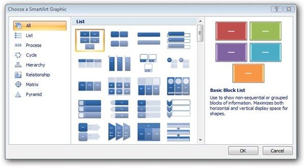
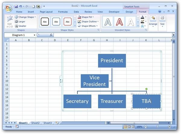
Select the particular graphic that you want to use and click OK. As an example, we’ll select the Organization Chart from the Hierarchy category.

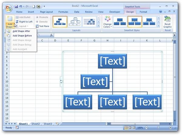
After clicking OK, you’ll be returned to the Excel spreadsheet with the SmartArt chart inserted. Additionally, two new tabs will appear on the Excel ribbon under the heading SmartArt Tools. By default, the Design tab will be open. On this tab, you can change the color, shape, and layout of the newly created chart. This is also the tab to go to if you want to extend the chart by inserting additional elements. To do this, just click on the Add Shape button in the Create Graphic category.
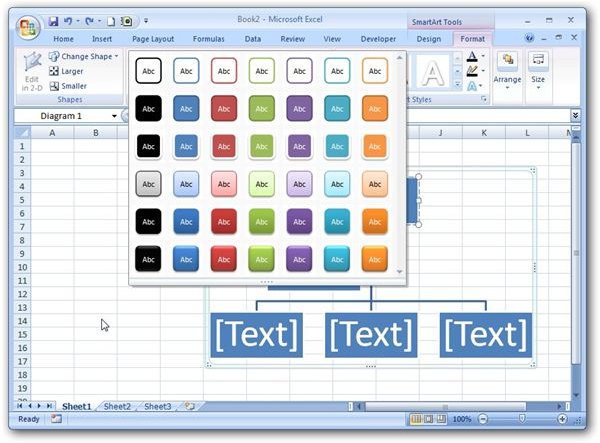
A number of other modifications can be made to the SmartArt chart from the Format tab on the Excel ribbon. Here, you can change the appearance of the individual blocks that make up the chart and make modifications to the text that appears in each block in addition to several other things.
When you’re ready to start filling information into the SmartArt object, just click on any of the blocks and begin typing. Don’t worry about changing the font size at first – that’s one of the “smart” things about SmartArt. The font will automatically adjust itself as you type so that your entire text message will fit in the block.
After you’ve entered all of your information and made any format and design changes, you can return to the main portion of the Excel spreadsheet by clicking anywhere else on the sheet. Note that this will cause the SmartArt tabs on the ribbon to disappear. You can access them again, at any time, by clicking on the SmartArt object.
Additional Resources: For more tips and tricks, be sure to take a look at the other Microsoft Excel tutorials and user guides available here on Bright Hub’s Windows Channel. Find new tips for designing charts and graphs , information on macro settings , and more. Additional articles are being added all the time, so make sure to check back often.


