The R1C1 reference style is an alternate way to designate worksheet cells. Read on to find out how to switch between this style and the standard A1 style in Excel if you suddenly find that all your column letters have changed to numbers.
Column Letters Changed to Numbers?
Problem: All of a sudden, the column letters along the top of your spreadsheet have been replaced by numbers, as shown in Fig. 197. (Click any image for a larger view.)
None of the formulas that you enter will work. What should you do?
R1C1 Reference Style
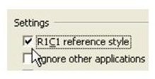
Relax. There are two ways of naming cells. Someone has turned on the R1C1 style of addressing. To return to the normal A1 style of cell addressing, go to Tools – Options. On the General tab, uncheck the box for R1C1 Reference Style, as shown in Fig. 198.
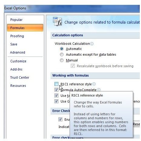
Alternatively, if you’re working in Excel 2007 or later, click the Office button in the upper left corner of the application and select Excel Options. Then select Formulas from the left menu and uncheck the box next to R1C1 reference style.
But wait – while you are here, you can learn something fascinating about spreadsheets. In the topic Copy a Formula That Contains Relative References , I suggested it was miraculous that Excel could automatically change a formula as you copied it. If you take two minutes to learn about this other method of cell addressing, you will understand that it may not be so amazing after all.
When Dan Bricklin and Bob Frankston invented VisiCalc, they used the A1 style of cell naming. When Mitch Kapor started selling Lotus 1-2-3, he used the same style. When Microsoft came out with their first spreadsheet product – Microsoft Multiplan – they used a very different method of cell addressing. This method is known as R1C1. In the Microsoft system, the rows are numbered just as in the A1 system. However, the columns are also numbered. Each cell is given a name, such as “R4C8”.
This name stands for the cell at Row 4, Column 8. This is the cell that you and I know as H4.
In the R1C1 style, the formulas are interesting. Look at this formula in cell D6, as shown in Fig. 199.
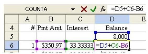
The formula in the formula bar says =D5+C6–B6. But when you think about this formula in plain language, what it is really means is “Take the cell just above me, add the interest in the cell just to the left of me, and subtract the payment in the cell two cells to the left of me.”
Formulas in R1C1 style are more like the plain language description above. If you want to enter a formula in D6 that points to the cell just above, it would be =R[–1]C. The number in square brackets after the R indicates to how many rows ahead or back you are referring. In our case, row 5 is one row above row 6, so you would put a –1 in the square brackets.
There is no number after the C portion of the address, which means that you are referring to the same column as the cell that contains the formula.
If you want to refer to a cell that is two cells to the left of the cell with the formula, you would use =RC[–2].
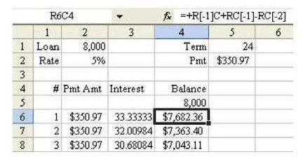
As shown in Fig. 200, the formula from Fig. 199 can be restated in R1C1 style as follows:
=R[–1]C+RC[–1]–RC[–2]
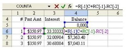
So, all relative references in R1C1 style have a number in square brackets, either after the R or after the C or both.
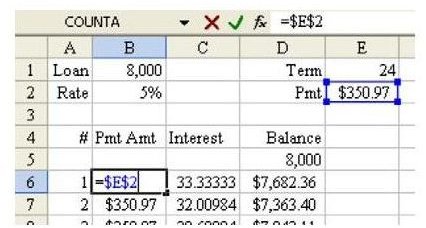
It is very interesting to see how this style does absolute addresses. As shown in Fig. 201, the formula in B6 is an absolute formula that always points to cell E2. The formula in A1 style is =$E$2.
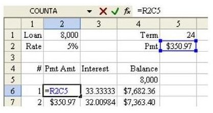
To enter a similar absolute reference in R1C1 style, you do not include square brackets in the address. As shown in Fig. 202, a formula of =R2C5 will ALWAYS point to cell E2.
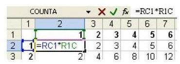
It is also possible to have mixed references. Flip back to Fig. 177 in the multiplication table topic . Fig. 203 shows that formula in R1C1 style:
Additional Details on R1C1 Style Formulas
Now that you understand the basics of R1C1 style formulas, you can appreciate the amazing part. Remember that Microsoft invented this method for their Multiplan product. Lotus 1-2-3 was the dominant spreadsheet in the late 1980s and early 1990s. Microsoft was battling for market share. Everyone using spreadsheets was familiar with the A1 style. No one would want to learn the R1C1 style in order to switch to Microsoft. So, in their Microsoft Excel product, they developed an elaborate system to actually store the formulas in R1C1 style, but then to translate the R1C1 formulas to A1 style to make it easier for all the Lotus fans to understand. By default, Microsoft starts with the A1 style addressing. However, you can remember from Fig. 198 that you are just one checkmark away from switching back to R1C1 style addressing.
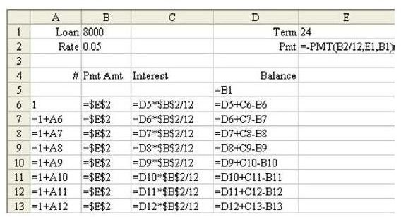
Finally, here is the amazing part. Examine the amortization table example in Formula View mode. (Hit Ctrl+~ to toggle into Formula View mode.) The Formula View mode in A1 style can be seen in Fig. 204. Every formula in column D is different.
The Formula View Mode in R1C1 style can be seen in Fig. 205. In A1 style, it seems AMAZING that Excel can change a reference from D10 to D11 when the formula is copied down. However, look closely at the formulas in each row of rows 7 and higher in the R1C1 style shown in Fig. 205. Each formula in a column is identical to the formula located just above it!
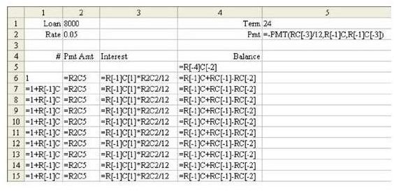
While VisiCalc and Lotus 1-2-3 made the formula replication seem amazing because of their A1 reference style, if the Multiplan invention of R1C1 style had taken hold, it would not seem amazing at all because, in fact, every formula is exactly identical as you copy it down through the rows.
If you ever plan on writing VBA macros in Excel, it is important to understand the R1C1 style of formulas. For general use in Excel, you never really need to totally understand the R1C1 style, but it is interesting to see how Microsoft’s R1C1 style is actually superior to A1 when copying formulas in a spreadsheet.
Summary: Learn R1C1 style formulas to better understand how formulas are replicated across a worksheet.
Commands Discussed: Tools – Options – General
More Excel Tips
If you’re interested in more tips and tutorials, be sure to check out the other Microsoft Excel articles available at Bright Hub, including: