Problem: You want to create two dropdown lists. The second list should be dependent on what is selected in the first cell.
Strategy: Use the INDIRECT function as the source of the second list.
Follow these steps:
-
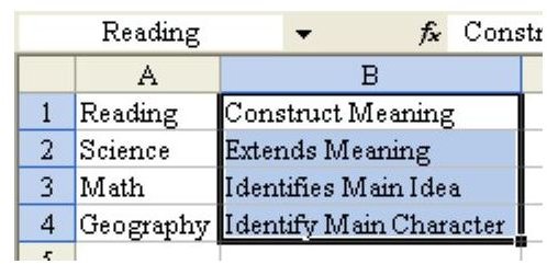
On a blank sheet, set up a list of items for the first dropdown: Reading, Science, Math, and Geography. Name the range “Subjects”, as shown in Fig. 1501.
-
In another column, set up a list of choices available for reading.
Advertisement -
Name this list Reading, as shown in Fig. 1502.
-
Repeat Step 3 for each item in list 1, as shown in Fig. 1503. In each case, the name of the new range must match the value in column A.
Advertisement
-
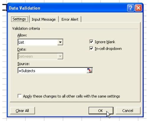
Set up the first dropdown list, where users will pick the subject. Select the cell. From the menu, select Data – Validation. Change the Allow box to be List; in the Source box, type =Subjects, as shown in Fig. 1504.
-
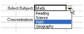
When you choose OK, cell D2 will have a dropdown list of subjects, as shown in Fig. 1505.
Advertisement -
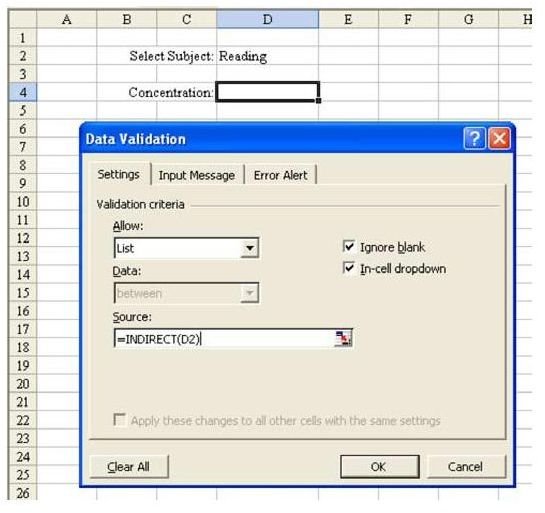
To set up the second dropdown, select cell D4. From the menu, select Data – Validation. Change the Allow: dropdown under Validation Criteria from Any Value to List. In the Source box, enter this formula: =INDIRECT(D2), as shown in Fig. 1506.
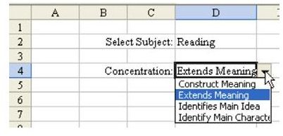
Result: When you select a value in D2, the formula for the second dropdown list will automatically update, as shown in Fig. 1507. The INDIRECT function looks in D2 and hopes to find a formula there. When they select Reading in D2, then the validation formula becomes =Reading. Since you cleverly set up a named range called Reading, Excel is able to populate the list.
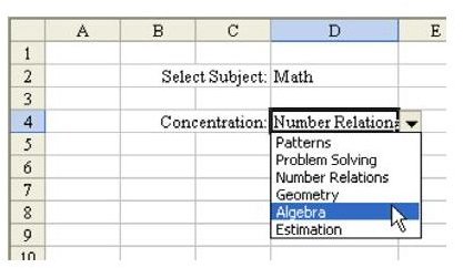
When you change D2 to be Math, the =INDIRECT(D2) will become =Math. Again, since you have a named range called Math, Excel is able to fill in the second dropdown with Math subjects, as shown in Fig. 1508.
Summary: Using the INDIRECT function as the formula in the List for Data Validation will allow you to set up a second validation list that is dependent on the choice in the earlier list.
Commands Discussed: Data – Validation
Functions Discussed: =INDIRECT()
Images