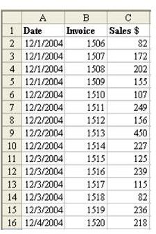
Problem: The owner of a retail store offers a five percent bonus when sales for a day exceed $1,000. In the dataset shown in Fig. 1315, you want to color all cells that are eligible for the bonus.
Strategy: In this case, you want to use SUMIF to keep a running total of all rows above the current row. If those rows are over $1,000, then the current row is eligible for the bonus.
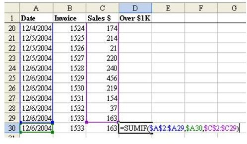
- It is easier to understand this formula if you enter it on the last row of the dataset, as shown in Fig. 1316.
This formula is similar to the formula in the last example, with one crucial difference. In the last example, the first and third ranges were examining all of the rows from A2 to A30 every time. This time, the top of the first range is locked at $A$2, but the bottom of the range is pointing to the row above the current row. The $A29 reference says that we are always looking at column A, but the reference will change to reflect the row above the current row.
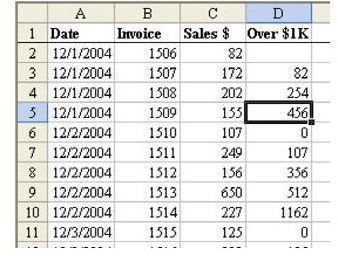
- Copy D30 up to all of the other rows. This formula does not work in the first row of the dataset, so leave cell D2 blank, as shown in Fig. 1317.
The formula keeps a running total of all prior sales that day. In cell D5, the $456 means that the three prior sales of $82+172+202 totaled $456. In Fig. 1317, the bonus program would only kick in on the sale made in row 10.
-
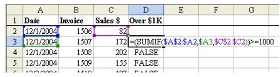
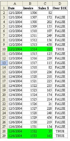
Edit the formula in D3 and add a test to see if this result is greater than or equal to 1000. You will have to add a leading parenthesis at the front and add )>=1000 at the end, as shown in Fig. 1318.
-
Copy this formula down and you have a formula that evaluates to TRUE or FALSE. The True values are sales eligible for the bonus.
Advertisement
You now want to set up the conditional format. Follow these steps.
-
It is easiest if you copy the formula that is working. Go to cell D3. Hit the F2 key to put the formula in Edit mode. In the formula bar, drag to highlight the entire formula.
Advertisement -
Hit Ctrl+C to copy the formula from the formula bar. Copying from the formula bar allows the text of the formula to stay on the clipboard after you hit the Esc key.
-
Hit the Esc key to exit Edit mode.
Advertisement -
Select cells A3:C30.
-
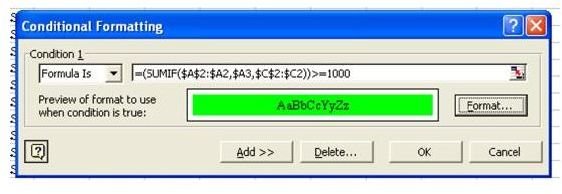
From the menu, select Format – Conditional Format. Use the dropdown to change “Cell Value Is” to “Formula Is”.
Advertisement -
Click in the Formula box, and hit Ctrl+V to paste the formula from the formula bar, as shown in Fig. 1319.
-
Choose the Format… button. Choose Green on the Patterns tab. Choose OK to close the Format Cells dialog. Choose OK to close the Conditional Format dialog.
Advertisement
Result: Sales that occurred after $1000 in sales for a particular day are highlighted in green, as shown in Fig. 1320. You can now safely delete your temporary formula in column D.
Summary: By changing the Conditional Formatting dialog from Cell Value Is to Formula Is, you can create amazingly powerful formulas to highlight entire rows if some condition is true.
Commands Discussed: Data – Conditional Format
Functions Discussed: =SUMIF()
Images