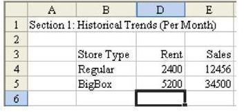
Problem: You have data hidden in column E, as shown in Fig. 1231. You want to quickly view data in the hidden column without actually unhiding it.
Strategy: Use this trick to temporarily view a hidden column. Note that this trick only works if you use Transition Navigation Keys. If you regularly work with hidden data, this cool trick might be enough to tip you over to turning on this setting.
-
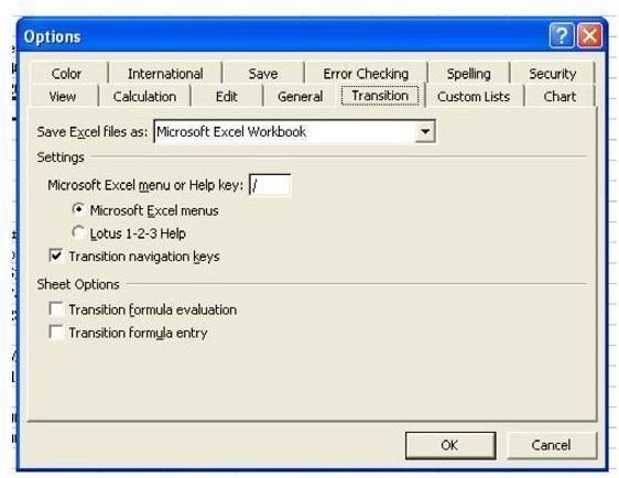
From the menu, select Tools – Options. On the Transition tab, choose Transition Navigation Keys, as shown in Fig. 1232. (Click any image for a larger view.)
Advertisement -
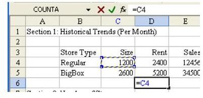
In the image, column C is hidden. Place the cell pointer in column D, in a blank cell. Type the Equal sign to start entering a formula.
-
Hit the Left Arrow key as if you were going to enter a formula using the arrow keys. Excel magically unhides the hidden columns, as shown in Fig. 1233. You can now arrow through the worksheet to look at hidden data.
Advertisement -
When you are done, hit the Esc key to cancel entering the formula. The hidden ranges will be hidden again.
Gotcha: Beware, users could employ this method to see hidden data. To avoid this behavior, you need to protect the worksheet.
Gotcha: This behavior can be incredibly annoying. If you are in cell D3 and hope to enter a formula of =2*A3, you might think this is only five keystrokes: =, 2, *, Left Arrow, Enter (a total of five strokes) However, when you actually try to do this, after the fourth keystroke the hidden columns will open. You usually just catch this out of the corner of your eye, as you incorrectly enter =2*D3 in the formula.
Summary: To quickly view hidden data in a worksheet, select a cell in the column to the hidden data’s immediate right, type an Equal sign, and then hit the Left Arrow key.
Commands Discussed: Tools – Options – Transition
Images