When creating an Excel formula, you can use the dollar sign to indicate an absolute or a mixed cell reference. In this tip, Mr. Excel explains a simpler way to insert a dollar sign when constructing these types of formulas.
Dollar Signs in Formulas
**
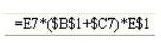
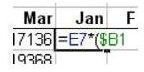
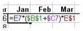
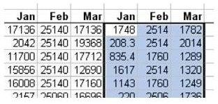
Problem: It is a pain to type the dollar signs in complex formulas such as the formula shown in Fig. 182 to the right. (Click any image for a larger view.)
If you’ve been thinking to yourself, “There must be an easier way to do this!”, you’re right. Find out this simpler method for adding dollar signs to cell references in formulas in the next section.
An Easier Way
Strategy: Use the F4 key as you are entering the formula. The F4 key will toggle a reference through the four possible reference types.
-
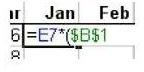
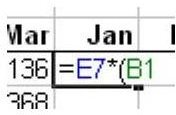
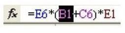
As shown in Fig. 183, start to type the formula =E7*(B1.
-
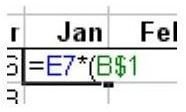
Immediately after you type B1, hit the F4 key. Excel will insert both dollar signs in the B1 reference, as shown in Fig. 184.
Advertisement -
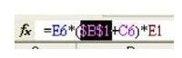
As an illustration, hit the F4 key again. Excel changes from an absolute reference to a mixed reference, with the row portion of the reference locked, as shown in Fig. 185.
-
Hit the F4 key again. Excel changes to a mixed reference, with the column portion of the reference locked, as shown in Fig. 186.
-
Hit the F4 key once more. Excel changes back to a relative reference, as shown in Fig. 187.
Advertisement
An Example
Here are the steps for entering the complex formula shown in Fig. 182.
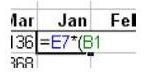
Step 1: Type =E7*(B1.
Step 2: Hit the F4 key once.
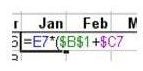
Step 3: Type +C7.
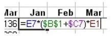
Step 4: Hit the F4 key 3 times. Your formula will now appear as shown in Fig. 188.
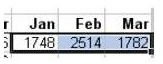
Step 5: Type the parentheses, an asterisk for multiplication, and E1, as shown in Fig. 189.
Step 6: Hit the F4 key twice to change E1 to a reference with the row locked, as shown in Fig. 190.
Step 7: Hit Ctrl+Enter to accept the formula without moving the cell pointer to the next cell, as shown in Fig. 191.
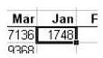
Step 8: With the mouse, grab the Fill handle (the square dot in the lower right corner of the cell) and drag it to the right for two cells, as shown in Fig. 192.
This will copy the formula from January to the other two months, as shown in Fig. 193.
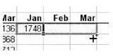
Step 9: Double-click the Fill handle. This will copy the three cells down to all of the rows with data, as shown in Fig. 194.
Additional Information: You might find mixed references confusing. As you work on building the first formula, you might know that you need to point to C7. Enter C7 in the formula and then use F4 to toggle between the various reference types. Say to yourself, “OK. There is a dollar sign before the C that will lock the column and let the row change – is that what I need?” As long as you say this to yourself without your lips moving, your officemates won’t think any less of you.
Further Information: If you did not add the dollar signs as you typed the formula, you can still use the F4 trick later. Using the mouse, highlight the proper reference in the formula bar, as shown in Fig. 195. After the reference is highlighted, you can hit the F4 key to toggle that particular reference through the four states, as shown in Fig. 196.
More Excel Tips
For more Excel tips and tricks, be sure to check out the other items in Bright Hub’s extensive collection of Microsoft Excel tutorials. In particular, you may be interested in the following selections.
91 Tips for Calculating with Microsoft Excel – This collection of tutorials, written by Mr. Excel himself, contains detailed explanations and useful tricks for getting the most out of Excel’s calculation abilities.
Excel Formatting Tips from Mr. Excel – In addition to demonstrating how Excel’s formatting capabilities can be used to make a spreadsheet more visually appealing, this set of 72 tips and tricks shows how to use the application’s built-in formatting features to make it easier to organize and analyze data.