
“Excelerate” your accounting tasks by learning how to make a loan amortization table in Excel. The advent of this excellent tool makes the process of keeping subsidiary ledgers easier. Use the guidelines furnished below and be surprised that creating a schedule is quick and trouble free.
Revisiting the Traditional Method of Maintaining Subsidiary Ledgers
Do you still keep tabs on receivables, using index cards instead of Excel spreadsheets that calculate automatically?
In this day and age of computerization, it’s quite surprising that the tickler filing system is still being used for bookkeeping purposes. For the benefit of those who are not familiar with this filing technique, it’s a system that utilizes 3 x 5 index cards as subsidiary ledgers . The said cards are used for monitoring individual account balances of customers’ receivable accounts, or depreciation expenses, expense amortizations and similar items. Typically, the transactions involve repetitive calculating tasks throughout the accounting cycle.
But posting errors are likely to happen as the task gets to be boring and monotonous. Procedural computations repeated several times over for a single account often lead to mistakes by picking up the wrong balance or by miscalculating the number of days–more so, if you have to repeat the same process for numerous individual accounts
If software is still beyond your capability or quite expensive in your region, why not learn how to create a spreadsheet wherein each cell is integrated with formulas that automatically calculate the cell values? One good example is a loan amortization schedule, and this article will give you guidelines on how to make an amortization table using Excel.
Guidelines for Creating a Schedule of Payments for Individual Loan Accounts
Monthly amortizations for long-term loans comprise monthly installment payments and the interest applicable on the outstanding balance for a specific period. Hence, the data you need to input are the following:
- Date the loan was released
- Principal amount
- Interest rate
- Amount of monthly installment
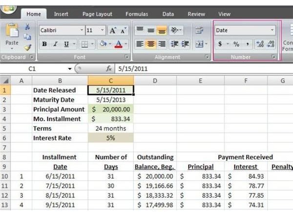
View our screenshot image for our sample amortization schedule and take note of the following when making your own inputs. Better yet, you can download a copy from Bright Hub’s Media Gallery so you can study the formulas more closely. (You will find a link in the last section on page 2 of this article).
1. Format the cells for your numeric data by selecting the “Custom” category and select the appropriate presentations, i.e. “Date” or “Accounting” or “Percentage," whichever is applicable. This is quite important since the spreadsheet will use numeric rules when working on these inputs.
2. For the benefit of those who are not too familiar with the Excel tools , click on the image to get a larger view of the sample — take note of the header and find the tool bar for number format highlighted inside a red square.
3. List downward the number of installment payments for the account you are working on under column A. Since our example is a long-term loan for two years, which is equivalent to 24 months, column A from Cell 10 to Cell 33 were used to index the corresponding order of amortization payments.
4. Create the headings for the following:
- Cell B8-9: Installment Date
- Cell C8-9: Number of Days
- Cell D8-9: Outstanding Balance, Beginning
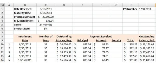
- Cell E8-F8-G8: Payment Received
- Cell E9: Principal
- Cell F9: Interest
- Cell G9: Penalty
- Cell H9: Total
- Cell I9: Outstanding Balance, End
5**. Installment Date –**
Type the monthly due dates for every installment payment under column B, starting with Cell B10 through Cell B33. The installment dates in our sample schedule commences on June 15, 2011 since the loan was released on May 15, 2011. Check if the 24th installment date is the same as your maturity date.
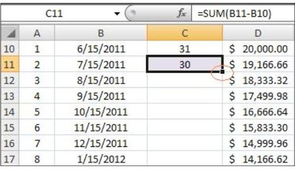
6. Number of Days –
The inputs under this column will be used for computing the monthly interest automatically. Nevertheless, you don’t have to count the number of days, because the following steps will lessen the tediousness of the process. In addition, it ensures that the days counted are accurate. Proceed by typing the following on the formula bar:
-
C10 =SUM($B$10-C1) – In order to come up with the number of days from May 16 to June 15, 2011, the spreadsheet tool has to deduct the 15 days that have already transpired from May 1-15. Otherwise, the entire 31 days for the month of May plus the 15 days for June will have a total of 46 days.
Advertisement -
C11 =SUM(B11-B10) – The next cell has a different procedure because we need to count from another date and deduct the number of days that have elapsed. This time, however, the adjustment is retrieved from the previous cell, which is Cell B10. We will call this our “parent formula,” since you will use it to create the same rule for the rest of the cells from C12 to C33.
-
The fun part in creating this schedule is that you don’t need to type formulas repeatedly. Simply click on the “parent formula” for this column, found under C11. Point the cursor at the bottom right corner and drag it down through Cell C33, and then press “Enter.” The cells will self-adjust by mimicking the rule you applied under Cell C11. View the screenshot images of our sample where you will find that the rest of the cells under column C automatically returned with their own corresponding number of days.
-
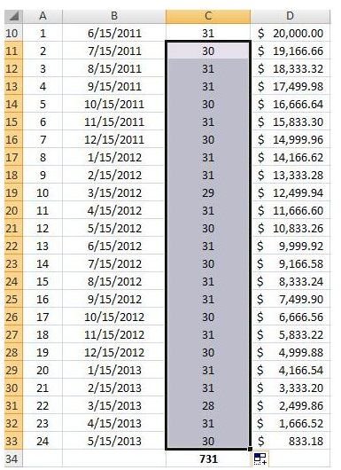
However, it would be best to check your number-of-day inputs from Cell C10 to C33 by footing the total against the total number of days of your loan duration. Since our example duration is for two years, the total number of days should be 730 (365 x 2). Notice, however, that our total number of days is 731, primarily because 2012 is a leap year, which the Excel program took into consideration.
Advertisement -
To prove your totals, use Cell C34 and type in the formula =SUM(C10:C33) on the bar. This denotes that values starting from C10 through C33 are summed-up. The autosum function will not work here because C10 has a different rule.
7. Payment Received – Principal
We will skip Column D, because the inputs here will be automatically generated by the spreadsheet. Hence, our attention will be on Column E, which will be quick and easy. You can simply copy-paste the equal-monthly amortization from E10 through E33. However, be alert of those instances when borrowers do not make the exact installment payment due; hence, you will have to modify the cell’s input for payment received accordingly.
Moreover, there may be some rounding-off adjustments, which you can put into effect in the last cell. As illustrated by our example, amortization for E33 is $833.18 instead of $833.34 in order to zero-out the outstanding balance under column I. Determine the amount of round-off adjustment by extracting the total of Cells E10 to E33. This time, you can simply highlight the said cells and make use of the auto sum function.
Kindly proceed to page 2 for the rest of the guideline on how to make a loan amortization table in Excel
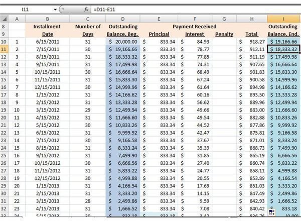
8. Outstanding Balance
Our first objective is to determine the figures for outstanding balances after every installment payment is made. Long-term loans make use of the diminishing balance as base or principal amount for purposes of interest calculations.
Outstanding Balance, Beginning Cell D10 – type-in the principal amount of the loan as the value of this cell.
Fill in the rest of the cells from D11 up to D33 by encoding the rule =I10 on D11, and then drag down the formula through D33**.** This will prompt the cells to automatically copy whatever values are reflected under column I according to their corresponding cell numbers. Once you have completed the inputs for column I, the values will automatically appear in each of the cells used under D column.
Outstanding Balance, End Cell I10 – Input the formula =D10-E10, which is a command to deduct the 1st monthly installment payment from the principal.
Cells I11up to I33 will simply adopt the rule by performing the same procedure of dragging down the “parent-formula” found in Cell I10. The actions performed in each cell will generate the diminishing or reduced balances of the principal after each installment payment. The last cell, I33, should reflect a zero balance to indicate that the installment payments have been properly applied.
9. Payment Received – Interest

At this point, we are about to compute the monthly interests due on each installment payment. Recall that the formula for interest is the basic I = Principal x Rate x Time. For this purpose, however, the principal is based on the diminished balance; hence, the values used are retrieved from columns D and C. Encode the formula =(D10*$C$6)*C10/365 for Cell F10.Use the same rule by dragging this formula from F11 through F33, then press enter.
The rule is translated as— Outstanding Balance, Beg (D10) x 5% Interest rate (C6) x Number of days (C10) over 365 days. Take note that the dollar ($) symbol for C6 was used, because the value for this cell remains constant throughout the F columns from F10 to F33. Each of these cells now has the capability to generate the monthly interest due from the borrower.
10. Payment Received Total
This column automatically calculates the installment amount or monthly amortization payments due from the borrower, by encoding the formula =$E$10+F10+G10 on Cell H10. Use the same procedure of dragging down the rule down to H33.
11. Payment Received – Penalty
Use this column for any penalty charges due in the event that the customer defaults in any installment payment. Although the input will not affect the balances, it would be best to compute this item manually since the values are likely to vary.
12. The Downloadable Sample
Users may choose to utilize the sample we used to illustrate the guidelines on how to make a loan amortization table in Excel by downloading a copy at Bright Hub’s Media Gallery . One can simply modify the inputs specified in the earlier part of these guidelines. The cells with automated functions will work on the new data in accordance with the rules integrated in each unit to come up with the values. Still, it would be best to check them out randomly as well as prove the total of each column.
References and Image Credit Section:
Reference:
- The tutorial and its related guidelines were all based on the author’s expertise as a former branch accountant of a universal bank.
Image Credits:
- Lisamarie Babik/Wikimedia Common
- Screenshot images created by the author.