Stocks have rallied from a long-overdue pullback after a ten month rise from the March, 2009 bottom. Are stocks going even higher? Are they ready to resume the pullback? One of the ways to determine if a financial vehicle such as stocks, bonds, gold, oil, is at an extreme value is Bollinger Bands.
Bollinger Bands Introduced
What are Bollinger Bands? We have all heard the age-old market bromide: buy low, sell high. Sounds simple enough. Until you start trying to figure out just how low is “low” and how high is “high”. High and low are relative terms, usually in reference to some norm. But what if the norm itself varies over time? Now what are high and low? Bollinger Bands is among the newer tools to help us figure this out.
What They Are
Attempts to answer the questions that we posed above led to the development of “envelopes” when analyzing financial securities. As a security’s price varied, how could one determine when the security’s price reached an extreme high or low that wouldn’t, or couldn’t, be sustained. Some of the early work used moving averages that were adjusted up and down by a fixed value or percentage. The next refinement was to find a way to have “adaptive bands” where the price action of the security determined the band values. Such a technique would attempt to enclose a high percentage of the overall data. This method used a 21-day simple moving average and would include 85% of the data. Thus, the moving average was moved up by 3% and down by 2%. These became known as Bomar Bands, whose creator, Marc Chaikin, worked for Bomar Securities at the time.
Bollinger Bands emerged in the 1980s when John Bollinger was trading warrants and options. After examining several statistical methods, he landed on standard deviation. Okay, now; don’t run away shrieking. Yes, we mentioned statistics and standard deviation in one sentence. Be brave. You will see that this is just a fancy name for some not-so-fancy arithmetic.
A Little Side Trip To A Not So Scary Neighborhood
Let’s look at some simple numbers: 6, 13, 15, 21, 32, 33, 42. Now let’s compute the average, also called the “mean”:
Avg = 6 + 13 + 15 + 21 + 32 + 33 + 41 = 161/7 = 23
One of the questions you could ask about this set of numbers is, “How closely are these numbers gathered around the average?”. One of the ways to figure this out is to compute the distance from each number to the mean:
6 - 23 = -17
13 - 23 = -10
15 - 23 = - 8
21 - 23 = - 2
32 - 23 = 9
33 - 23 = 10
41 - 23 = 18
We’ve got negative and positive values. If we just add these “distances” together, the negative values will cancel out the positive values and we won’t get the true accumulated distance of each number. If we square each of the values (remember, the square of a number is just the number multiplied by itself), we will then get all positive values because a negative number multiplied by another negative number yields a positive number.
-17 x -17 = 289
-10 x -10 = 100
- 8 x - 8 = 64
- 2 x - 2 = 4
9 x 9 = 81
10 x 10 = 100
18 x 18 = 324
Now we add up the squares:
289 + 100 + 64 + 4 + 81 + 100 + 324 = 962
and take the average:
962/7 = 137.52
By the way, the average-of-the-sum-of-the-squares of the distances (137.52 in this example) is called “variance” in statistics. Still, just simple arithmetic so far, right? One more step…take the square-root of the average, or variance, and you get 11.72. This final value is called “standard deviation”, and is represented by the Greek letter sigma. For the set of numbers in our exmaple, the standard deviation, or sigma, is 11.72.
Bollinger Bands and Standard Deviation
Now that we know about standard deviation, we can continue our explanation of Bollinger Bands. As we mentioned above, these bands are one of the ways to generate an “envelope” around the time variation of a given security price. Bollinger arrived at computing bands by taking a simple moving average (SMA) over a given interval, typically 50 days. To this average, he adds 2 standard deviations (called 2-sigma) of the 50 day’s data to get the upper band; he subtracts 2-sigma from the average to get the lower band. Simply put:
Bollinger Bands = 50-day SMA +/- 2-sigma
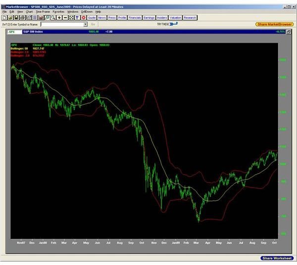
Here’s what Bollinger Bands look like in practice; this is a 2-year daily chart of the S&P 500 index with 50-day simple moving average with Bollinger Bands at 2.1-sigma. Bollinger’s website (https://www.bollingerbands.com ) recommends using 2.1-sigma when using a 50-day interval.
OK. So Now What?
We now have a reference for “high” (upper band) and “low” (lower band) relative to some normal value (moving average). We can refine our analysis to determine the most likely direction for the next price movement. We have to note here that the price merely touching one of the bands does not constitute a buy or sell signal. Nothing in life, or investing, is ever that simple. There are some additional indicators that we can compute from the bands that add insight into future direction; there are other technical analysis indicators that we can use along with the bands to generate buy and sell signals. In our next installment, we’ll look at these added calculations and indicators. Don’t worry; the calculations are even simpler than what we showed above.