Excel spreadsheets are a powerful tool that can calculate and display a lot of data quickly. Unfortunately, they can also become complicated and difficult to read. Conditional formatting is one way to improve Excel spreadsheets and make them more usable.
Conditional Formatting in Excel
Like all Microsoft Office applications, Microsoft Excel offers plenty of ways to format the data within them. Users can select different fonts, different font colors, different font sizes, and of course, use bold, italics, and more. The cells themselves can be edited as well with users able to select the background color of the cell, borders of various thicknesses, and even the type of data whether text, currency, dates, percentages, and more. The downside to all of this formatting flexibility is that a user can spend almost as much time formatting the data within a large and complex spreadsheet as they do entering in the data and building all of the formulas and calculations!
However, good use of formatting, data types and colors is critical for developing a spreadsheet that is easily readable by others and usable as a source of data and information. Fortunately, there is a way to format Excel spreadsheet data automatically.
Conditional formatting in Microsoft Excel automatically applies different formatting options to value, cells and data based upon various rules and conditions that can be set by the spreadsheet creator. In addition, several built-in conditional formatting rule sets are installed by default. Microsoft has made using Conditional Formatting easier in all versions of Office that include Excel, like Microsoft Office 2010 Home and Business .
How To Use Conditional Formatting
At first glance, using conditional formatting in Excel seems complicated. However, once you understand the basic concepts of how to use conditional formats, it becomes much easier and your spreadsheets will become more readable and better able to communicate the data to viewers.
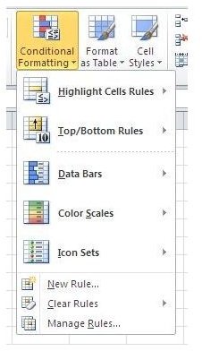
As with other formatting, the first step is to choose to which cells the formatting will be applied. Conditional formatting can be found on the Home tab under Styles. Choose which formatting condition to apply. In this example, we are formatting a small set of the “Germany” data so that those fields that are above the average are highlighted with red text on a lighter red background.

Those values that are above the average of the values selected are automatically highlighted without the user manually having to set those cells to be different colors.
Even better, once set, the conditional formatting stays in place for future updates to the data. For example, if the value of one of the cells is increased substantially, not only does it automatically become highlighted because it is above the average, but the color formatting is removed from previously highlighted values that are no longer above the average which has increased since the one value has gone up due to the increase.
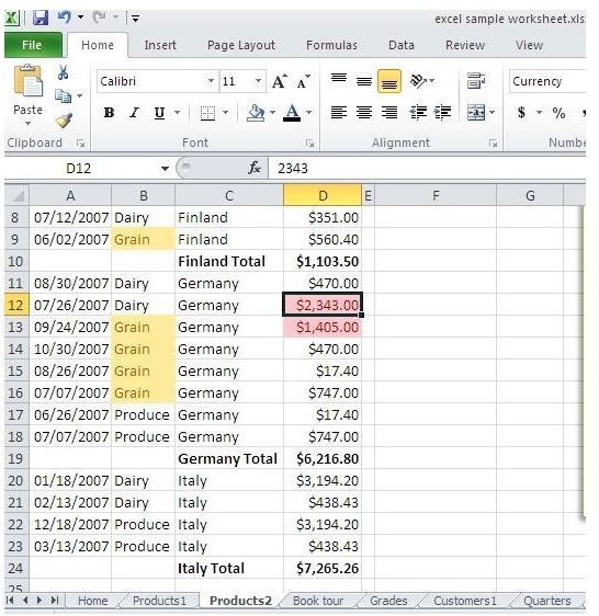
In addition to default conditional formatting, users can create their own conditional formatting triggers as well. Users can format data based upon numerous criteria using the conditional formatting tools that replace complicated formula building and scripting. In this example, cells that have the value Germany are highlighted in red.
Thanks to the simplified Conditional Formatting tools and the build-in formats, making Excel spreadsheets easy to read while spotlighting important data is easier than ever.


