How To Make A Thermometer Chart in Microsoft Excel 2010

Overview

You have something you want to track over the course of a few months and want a simple, effective way of keeping everyone in the loop. What should you do? In many circumstances, a simple rising thermometer chart made in Excel will serve your needs nicely.

A thermometer chart only keeps track of a single variable, whether it is a sales goal, fundraising goal, weight loss, number of cookies sold or customers retained. The thermometer is simply displaying a percentage of the goal. For example, if your sales goal is $1,000,000 and you have already made sales of $500,000, you could have a thermometer half-full showing you are at 50% of your sales goal.

With that out of the way, let’s get down to building our thermometer in Excel 2010. If you are using Excel 2007, the process is similar. There is an excellent article on BrightHub you can look at on how to create a thermometer chart in Excel 2007.

Setting up the spreadsheet

For the purposes of illustration, I’m going to make a thermometer chart showing how far we are to meeting a sales goal. You can use your own values and goal. Keep in mind that you don’t need to use multiple columns like I am going to do. The only piece of data you need is a single value - a percentage of your goal.

1. Open Excel 2010.
2. Column A will list out the number of months in a year (1-12). Column A will not figure into our formula, but will make it easier for the person updating the spreadsheet. Enter a label called Month in A1.
3. Column B will be our sales figures for each month. Enter in a few sales figures and label B1 with a label of Sales Made.
4. At the bottom of Column A, label the cell Total (A14). Cell A15 should be labeled Goal and A16 should be labeled Percent to Goal.
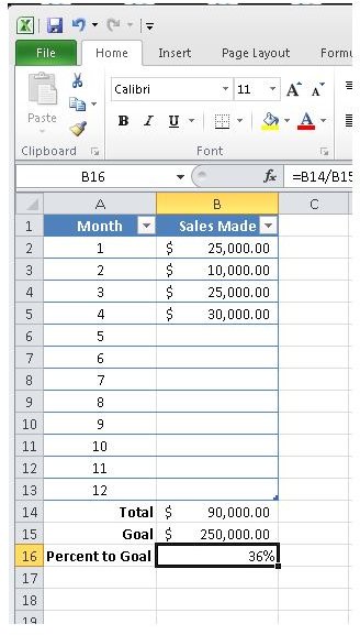
5. Create a simple formula for B14. It should be something like =sum(B2:B13). You should now have a total of the sales you entered into column B.
6. In B15, enter a sales goal.
7. In B16, enter a simple formula like =B14/B15*100. This will give you a percentage to use in the thermometer chart. This is known as your “key” for the chart.

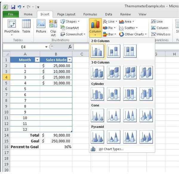
Stop for a second and make sure your table is set up properly. If you have been following along, your spreadsheet should look something like Figure 1. Next, we’ll use our percentage to create the thermometer.

Making the thermometer chart in Excel 2010

1. Click the Insert tab, navigate to Column, 2-D Column and finally the first 2-D chart called Cluster Column (Figure 2).
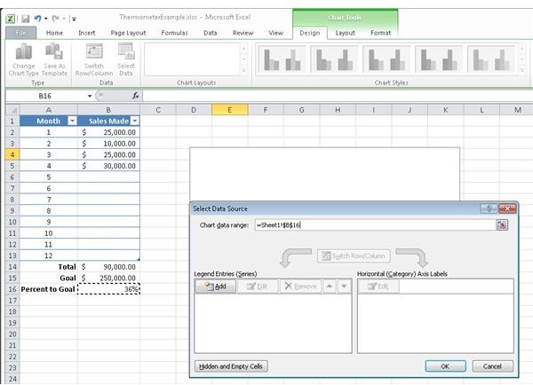
2. Click once in your (empty) chart and then click the Select Data button on the menu bar.
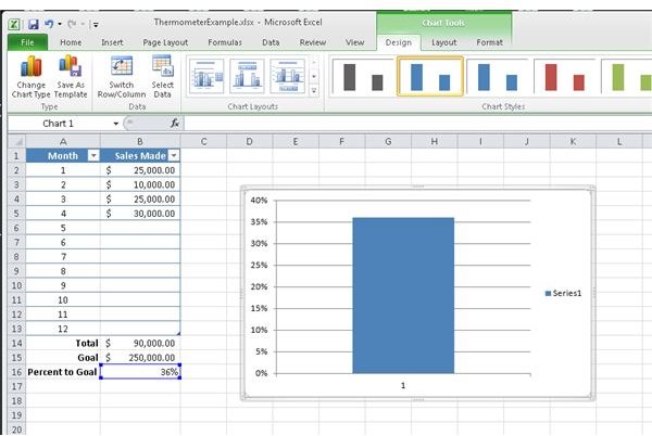
3. The Select Data Source dialog box will open. Click on cell B16 (your percentage for your goal) and click OK (Figure 3). You should now have a single column displayed in your chart (Figure 4).
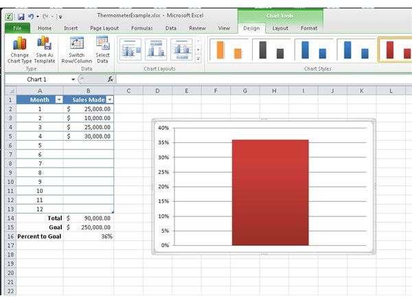
4. Make sure your chart is still selected and under Chart Styles select a color for your chart. Red seems appropriate.
5. Right-click on the text labeled Series 1 and select Delete.
6. Right-click on the label for the bar 1 and select Delete. Your chart should now look like Figure 5.
7. Right-click on the horizontal lines and select Delete. You should now just have a lone red bar along with the corresponding percentages along the y-axis.
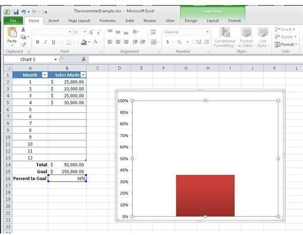
8. Double-click on the percentage along the y-axis. The Axis Options dialog should open.
9. Change the minimum and maximum numbers from Automatic to Fixed and enter 0 for minimum and 1.0 for maximum. Click OK. Your chart should look like Figure 6.
10. Click on the red bar and resize the bar so it is thinner – more thermometer-like.
11. Double-click on the chart. The Format Chart Area box should open. Click on Border Color and select No Line. Click Close.
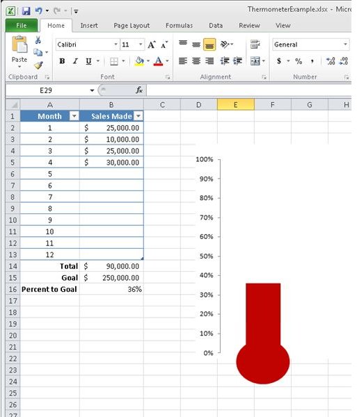
12. Next, draw a simple circle around the bar portion of our chart. Resize the circle and move it to the bottom of the bar chart. Be sure the circle is brought to the front of the bar chart. Also, change the color to match the bar chart.

Figure 7 shows the end product. With that, you should be done! Feel free to fancy things up a bit or even get ambitious and set your maximum percentage value from step 9 above higher than 100%. Good luck and I hope you not only meet your goal, but far exceed it!