Microsoft Excel 2007 is loaded with tools for creating, managing and viewing data. But Excel’s new interface makes using those tools easy.
Microsoft Excel 2007’s Parts and Functions
Microsoft Excel 2007 gives users state-of-the-art tools for creating, managing and presenting data. But Excel’s developers have made those tools easier to get to, compared to prior versions.
The Ribbon
A key graphical interface feature of Excel 2007 is the Ribbon, which is a toolbar that contains icons for the most common commands. Think of the Ribbon, which is new to Excel 2007, as a Turbo Toolbar: it speeds your workflow by enabling easy navigation to the tools you need. Unlike the old style menus, which you have to open each time you want to use a tool, the Ribbon’s toolbars stay exploded open.
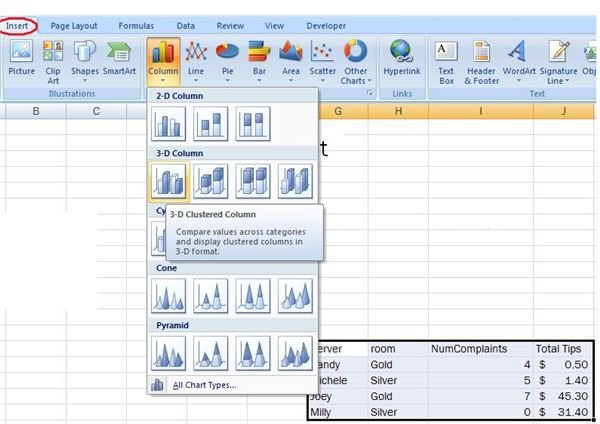
Watch the Ribbon in action: create a small table of data in a worksheet, then select the Insert menu tab. The Ribbon changes completely, filling its width with an array of objects that you can insert into a worksheet.
Click the Column icon to create a column chart. The drop-down menu displaying the sub-styles of Column charts is completely graphical, making short work of finding the style you need.
Choose any sub-style in the Column style. Notice that Excel refills the Ribbon with new tools – the ones you’ll now need to work with an existing chart. As before, these tools remain visible so you don’t have to dig for them in a collapsing drop-down menu.
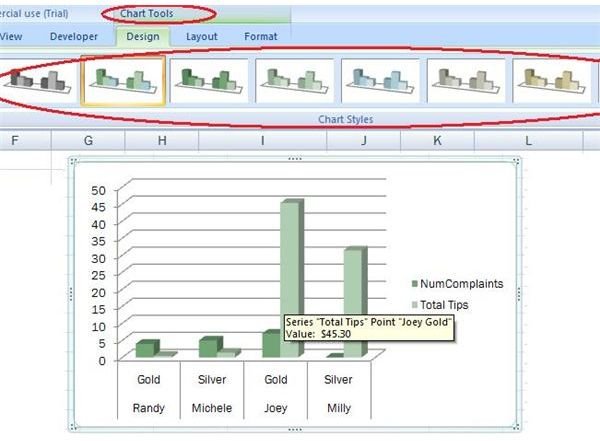
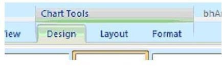
Notice that creating the chart has created an extra menu title, Chart Tools. If you navigate to another tab, you can quickly get back to the chart functions by single-clicking this Chart Tools heading.
Learn more about Excel’s Ribbon from the following two articles:
Customizing and Adding Buttons to the Excel 2007 Ribbon
What is the Microsoft Office 2007 Ribbon?
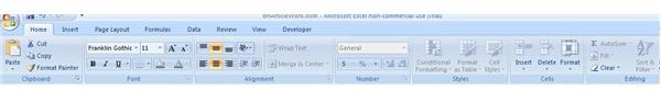
The Home Menu
The Home menu contains all the most commonly used functions and tools in Excel 2007. The copy and paste, text and number alignment, AutoSum, and find/replace tools are here – but notice that they have their own groups or panes: the Clipboard command group holds the clipboard tools, the Font group holds the font tools and functions, and so on, through the Editing group. The logical and graphical grouping of similar tools isn’t new to MS Office or Excel 2007, but the clarity of their icons is.
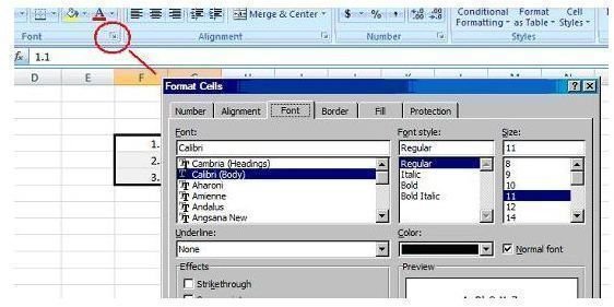
Keep in mind that the command groups display the most commonly used tools by default, but you still have quick access to the less commonly used tools and functions: on the Font group, click the small arrow, (called the Dialog Box Launcher) in the lower right hand corner. A dialog box appears to present more tools for managing fonts.
The clipboard viewer
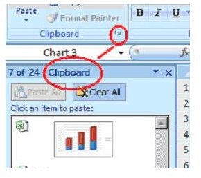
The Home tab’s Clipboard Viewer is a step up from the usual copy and paste tools. Clipboard Viewer lets you paste any of 24 clipboard items that you previously copied to the clipboard. Click on the Clipboard group’s dialog launcher to open the Clipboard Viewer. If you leave open the Clipboard Viewer and copy several worksheet cells to the clipboard, the clipboard viewer dynamically updates with each copy, displaying the source and content of the copied item – including graphics, if you copied a chart.
The Insert Menu
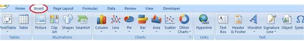
Selecting the Insert tab fills the width of the Excel 2007 Ribbon with icons whose tools and functions insert objects into worksheets.
One type of object is called SmartArt, which is new to Excel 2007. SmartArt is like an evolved version of the Shapes you can illustrate Word and Excel documents with. Use the SmartArt Picture Caption List, for example, as a storyboard to depict a narration.

The command groups Tables, Illustrations, Charts, Links, and Text hold other objects you an insert in worksheets.
With the Pivot Tables (in the Tables command group) you can quickly arrange lists and tables. Try out Pivot Tables with the following example.
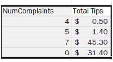
In a worksheet, enter the data shown in the table at left in this graphic:
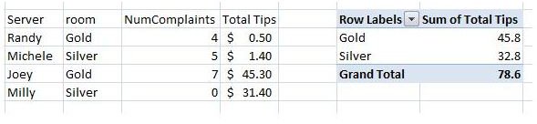
Select the table and then choose Pivot Table>Pivot Table on the Insert tab’s Table command group. In the Create Pivot Table dialog box, leave all options as they first appear, except for Existing worksheet. Choose that option, then select any blank cell in the worksheet. In the Pivot Table Field List that appears, select the Room and Total Tips checkboxes. The Pivot Table is created, displaying how many tips were collected, by serving room. You can easily reconfigure this table to display other data, by clicking the pivot table and changing which of the table’s fields are checked. Learn more about using Pivot Tables here:
Making and Using Pivot Tables in Excel
How to Manage Your Project’s Graphics with Excel

Choosing the Page Layout tab exposes tools for polishing your Excel 2007 worksheets for presentation. The Page Layout’s command groups are as follows:
- Themes, containing tools for unifying the look of your workbook
- Page Setup, for setting page margins, print areas and completing other printing-related tasks. You can choose a background image for your Excel 2007 document here.
- Scale to Fit, to size your worksheet’s content for printing
- Sheet Options, for toggling visibility of column and row headings and gridlines, both for printing and screen display
- Arrange, for toggling visibility and managing the layering of graphical elements like charts and SmartArt. You can also use the Arrange group to align and rotate some graphical objects like basic shapes.
Try this example showing how to bring one chart object in front of another:
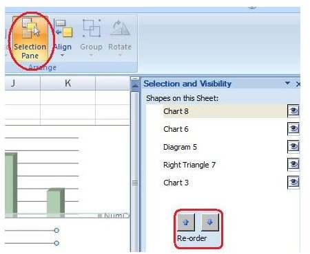
Create a small table of data, such as the one in the example in the Insert Menu section of this article. Create a chart from the table (Insert>Column, for example). After the chart is created, select, copy and paste it to duplicate the chart. Place the duplicate on top of the first chart, but so you can still see the first chart. Select Page Layout>Selection Pane. In the Selection and Visibility pane that appears, select the line representing one of the charts you made, then press the up or down Re-order arrows at the bottom of the pane until the partially hidden chart comes to the front to hide the other chart.
The Formulas Menu

Clicking the Formulas menu tab loads onto the Ribbon the functions and components you need to do computations on your data. Here are the command groups for the Formulas menu:
- the Function Library, with subcategories (e.g. financial, logical, data and time) of functions you can use to run calculations on your data.
- the Define Names group, which lets you create, for example, a name to refer to a table. By using names, you won’t have to use a hard-to-remember range name like “a5:d22”
- Formula Auditing, which lets you track down and validate the inputs to your worksheet’s functions.
- Calculation, which lets you specify when and how often worksheet functions get recalculated.
User Defined Functions
You can define your own functions in Excel 2007, and they’ll appear in the Insert Function dialog box under the category “User Defined.” Read Developing User-Defined Functions for Excel 2007 [https://msdn.microsoft.com/en-us/library/bb226683.aspx for details on how to create your own functions.
Example: Formula Auditing Functions
Try one of the formula auditing functions by doing the following: enter this function in a worksheet:
“=a1 + b2”
Then enter some numbers into cells a1 and b2. The formula displays the sum of a1 and b2. Select the cell containing the formula, and select the Trace Precedents tool in the Formula Auditing group in the Formulas menu. Excel 2007 will draw arrows from the formula to cells a1 and b2, showing you the cells your formula depends on to do its calculation.
Managing Your Data with Excel

The Data menu has tools for collecting, sorting and grouping data, and has these command groups:
- Get External Data: this group has tools for pulling data into Excel 2007 from a variety of sources, including the Web.
- Connection: this group lets you specify how often you want your imported data to be updated
- Sort & Filter: the tools here let you rank and sift through table data. Read details on Excel’s Filter tool here.
- Data Tools: these tools let you validate your data, and run calculations on tables on separate worksheets. Data Tools also lets you answer questions like, “If I know the result for the AverageOrders cell is 20, what can I change one of the individual orders to, to produce that average of 20?”
- Outline: the functions here allow you to group together rows or columns, so you can collapse (hide) or expand (reveal) them to better see the higher-ranked categories of your data as opposed to details.
Try the following example of using the Consolidate tool. This tool lets you combine tables on separate worksheets into one single table.
Create a table that looks like this:
Select the table and enter “a” in the Name Box to name the table. The Name Box is the text box just above the leftmost, top cell on your current worksheet.
Copy the table to another worksheet and change some of the data. Select the table and enter “b” in the Name Box. Imagine that the first table represents the data of one location of a restaurant franchise, and the second table is from another location in the same franchise.
On a new, blank worksheet, select the Consolidate tool from the Data menu, Data Tools group. In the Reference box, enter “a,” then click Add. Then enter “b” in the Reference box, and click Add again. Click the OK button to produce a new table that adds the data in the two source tables.
The Review Menu
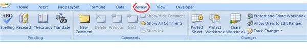
Excel’s Review menu has tool groups for spell-checking your workbook, adding comments to it, and locking it to prevent unauthorized changes to your data. The level of control you have here is considerable. For example, using the Allow Users to Edit Ranges tool, you can specify exactly which users on your network may modify data in your workbook. You can create such permissions down to the level of a worksheet cell, or any range of cells.
The View Menu

With the View menu you can work with tools for arranging windows, so you can see the data in your workbook clearly.
- Workbook Views: apply different views to your worksheets, e.g. a full screen view and print preview
- Show/Hide: expose or hide gridlines and column and row headings
- Zoom: zoom in or out on data
- Window: open new windows to view two distant parts of the current worksheet at the same time
- Macros: record scripts that automate Excel 2007
The Save Workspace tool is a time and work-saver if you work with several open workbooks at once. Clicking the Save Workspace tool saves the window layout for each workbook you have open. The next time you want to work with that same set of workbooks, using the same window layouts from the previous session, open up the Workspace file. Doing so saves you the work of having to open each workbook separately.
The Developer Menu
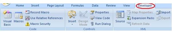
Excel 2007’s developer menu contains toolgroups to extend and automate Excel’s out-of-the-box functionality. Included here are tools to record macro scripts and import XML files. With the Controls command group, you can also add buttons to your worksheet, to call up custom forms for data entry or a macro script. Learn how to record a macro here.
Microsoft Excel 2007 puts together a large number of tools for collecting and managing data. But, the clear new interface shortens the learning curve for those tools.
References


