The split panes option in Excel 2007 allows you to view multiple areas of the same spreadsheet at the same time. Read on to find out how to activate this feature.
Sick of Scrolling Back and Forth?
One thing that many love about Excel is that you can almost always add a new row or column to a spreadsheet to keep track of additional information without losing the data that’s already there. There are times, though, when the spreadsheet can start to look cluttered, and all that information seems to get lost with the constant scrolling back and forth from one end of the document to another.
Sometimes, it is possible to move the information around so that all the pertinent facts are located close to one another on the spreadsheet page. However, that method isn’t always viable, especially if you’re dealing with a file that contains a database or a number of calculated formulas. One way to handle this problem is to use Excel’s split panes feature.
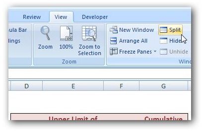
In Excel 2007, the Split Panes command is located on the View tab of the Excel ribbon in the Window category. If your Excel window isn’t maximized, you may have trouble spotting this command at first since it is one of the first ones to get truncated if there isn’t enough display room on the ribbon. If you’re having trouble finding it, the screenshot below shows the location of the command. (Click any image for a larger view.)
To use the command, just place your cursor on any cell that you want to use as the break point for the panes. Note that if you select a cell that is in the first row or column of your spreadsheet, then the split panes command will separate the page into two parts. However, if you select any other cell, the spreadsheet will be divided into four panes as in the screenshot shown below.
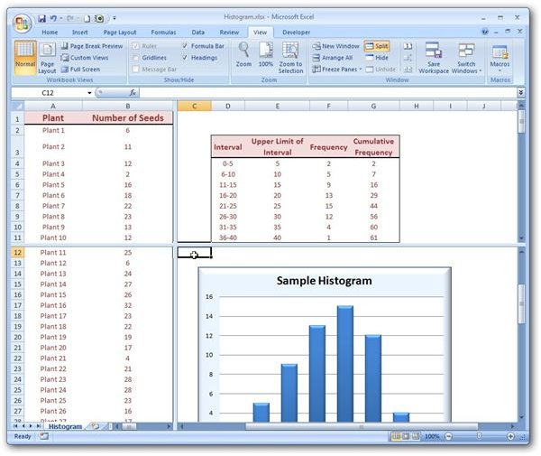
When activated, any of the panes can be scrolled separately without affecting the remaining ones. This can be very useful if you want to freeze a certain part of the spreadsheet or if you want to view the beginning and end of the same workbook page without physically moving the data.
To deactivate this feature, just return to the View tab and click the Split button again. This will cause all panes to be removed and the spreadsheet will be returned to its original state.
Note that when do use the split panes feature in a worksheet, each pane will contain the full worksheet. So, in essence, you’re really creating either two or four copies of the same information that you can scroll through as you wish. That is, this command is not really locking any of the cells – it’s just making it easier for you to view multiple areas of the sheet at one time.
For more tips and tricks, be sure to take a look at the other Microsoft Excel tutorials and user guides available here on Bright Hub’s Windows Channel. Find new tips for designing charts and graphs , information on macro settings , and more. Additional articles are being added all the time, so make sure to check back often.


