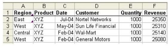
Problem: You need to create similar charts for each sales region from the transactional data shown in Fig. 994.
Strategy: There have been many pivot table examples in the book. It is also possible to make a chart that relies on a pivot table.
-
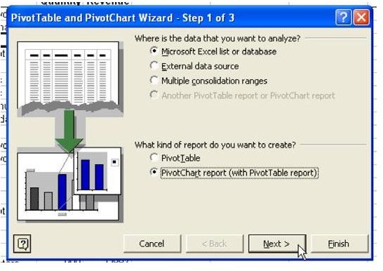
Select a single cell in your data and choose Data – PivotTable and PivotChart. In Step 1 of the Wizard, change the last option button to create a pivot chart, as shown in Fig. 995. Hit Next.
Advertisement -
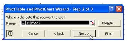
Confirm the data range in Step 2. Choose Next, as shown in Fig. 996.
-
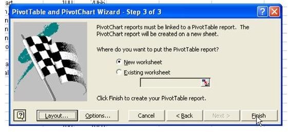
In Step 3, choose Finish, as shown in Fig. 997.
Advertisement
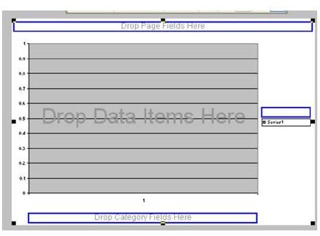
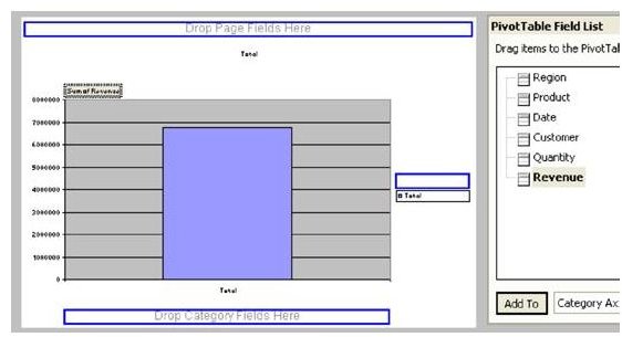
You will be presented with a blank pivot chart, as shown in Fig. 998.
- Drag the Revenue field from the Field list and drop it in the main part of the
chart, as shown in Fig. 999.
-
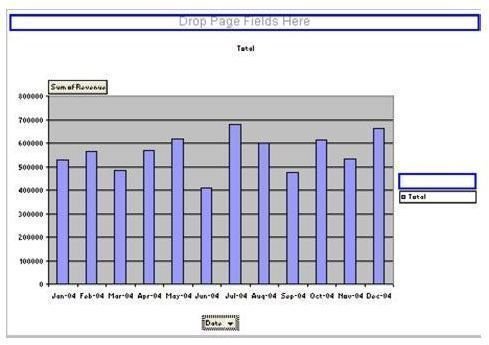
Drag the Date field and drop it in the Category Fields area, as shown in Fig. 1000.
-
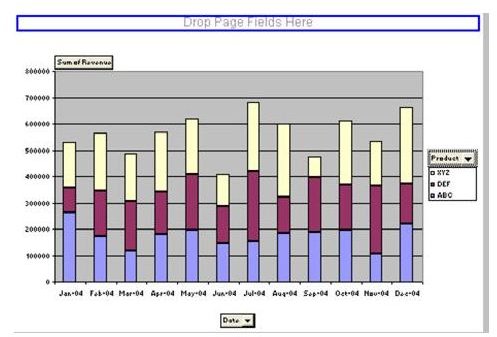
Drag the Product field and drop it in the blue box near the legend on the right side of the chart, as shown in Fig. 1001.
Advertisement -
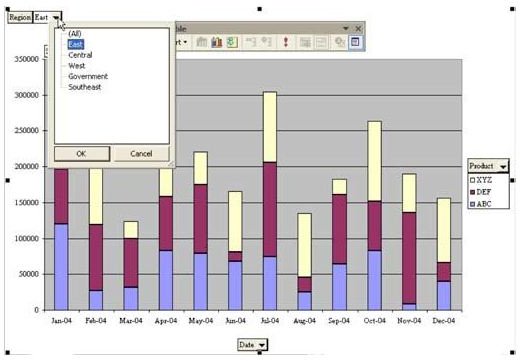
Drag the Region field and drop it in the Page Fields area.
Result: As shown in Fig. 1002, you can change the Region field to quickly produce a chart for each region.
Summary: You can use a pivot chart to create charts for several different regions.
Images