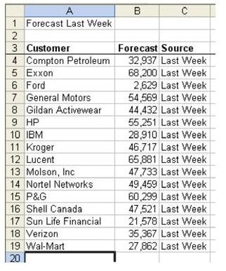
Problem: You have last week’s report of forecasted orders. You receive a new forecast report. As shown in Fig. 972, you need to determine which forecasts are new, which forecasts were changed, and which forecasts were deleted.
Strategy: Copy the two lists into a single list, with a third column to indicate whether the forecast is from this week or last week. Create a pivot table and the new/deleted/changed forecasts will be readily apparent.
Follow these steps:
-
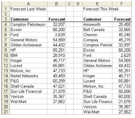
Add a heading in C3 called Source. Assign the value of “Last Week” in C4:C19, as shown in Fig. 973.
-
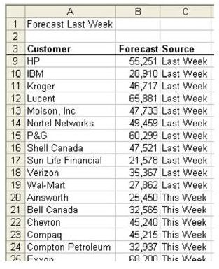
Copy the data from columns E and F to A20. In C20:C37, enter the value of This Week, as shown in Fig. 974.
Advertisement -
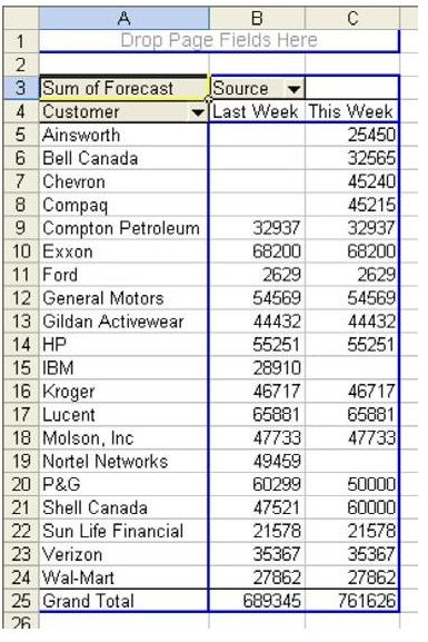
Create a Pivot Table. Put Customer in the Row area, Source in the Column area, and Forecast in the Data area.
-
In the PivotTable Options, turn off Grand Total for Rows. As shown in Fig. 975, you will have a comparison of the two lists.
Advertisement
Results: For any cells without an entry in Last Week, the forecast is new. For any forecast without an entry in column C, the forecast was deleted. For any forecast where columns B and C do not match, the forecast was changed.
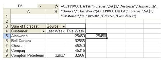
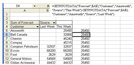
Gotcha: It would be nice to add a formula in column D that shows the difference between Last Week and This Week. However, if you use the method of highlighting a cell in the pivot table with the mouse or arrow keys while you enter the formula, Excel automatically changes the B5 reference to a GetPivotData function. Instead of getting a simple formula like =C5–B5, you get a complicated formula with GetPivotData formulas, as shown in Fig. 976.
As you copy this formula from D5 to D6, it does not have a relative reference. As shown in Fig. 977, the results will be wrong in the rest of the rows.
You have two options in order to enter a regular formula outside of the pivot table.
First option: You can actually type =D5–C5 as the formula.
Second option:
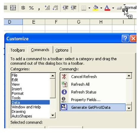
Alternatively, you can add a button to a toolbar to permanently turn off the automatic creation of GetPivotData functions. From the menu, select Tools – Customize. Choose the Commands tab. In the Category dropdown, choose Data. Scroll all the way to the bottom of the Commands list. There is an icon for Generate GetPivotData. Drag this icon from the Customize dialog and drop it on one of the toolbars, as shown in Fig. 978.
You can now turn off the creation of GetPivotData functions automatically by selecting the item in the toolbar, as shown in Fig. 979.
Summary: In addition to using VLOOKUP or Data Consolidation, you can use pivot tables as a quick way of comparing two or more lists. The trick is to add a new temporary column identifying the source of each record and then to use the Source column as a Column field.
Images