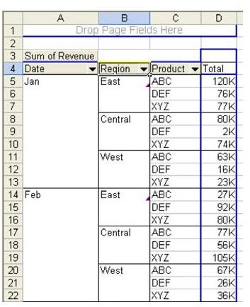
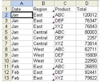
Problem: You have created a pivot table report and want to use this data as a database in another workbook. The pivot table report always uses this outline format. It may look great, but it is not conducive to data analysis. As shown in Fig. 963, you really need the Jan heading to be copied to A6:A13, and the East label to be in B6 and B7.
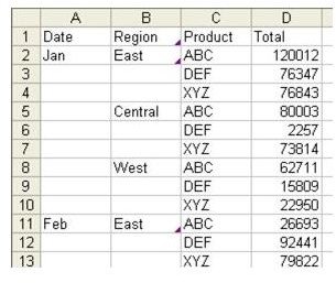
Strategy: To fill in the blank cells in the outline of the pivot table, you must make a valuesonly copy of the pivot table. Insert a new worksheet. Copy A4: D111 from the pivot table. On the new sheet, use Edit – Paste Special – Values in order to convert the pivot table to static values, as shown in Fig. 964.
In this case, you need to fill in the blank cells in columns A and B with the value from the cell above. Follow these steps.
-
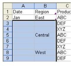
Select cells A3:B108, as shown in Fig. 965.
-
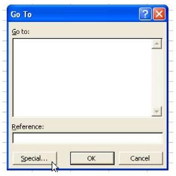
Press the F5 key to display the Go To dialog. In the lower left corner, choose the Special… button, as shown in Fig. 966.
Advertisement -
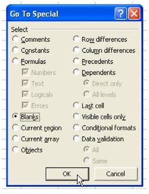
On the Go To Special dialog, choose Blanks from the first column and then choose OK, as shown in Fig. 967.
-
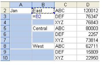
This next part is confusing, but it works. Type an Equal sign. Hit the Up Arrow, as shown in Fig. 968.
Advertisement -
Press Ctrl+Enter, and you get the result shown in Fig. 969.
Here is why this works. When you hit the Equal sign, you are telling Excel that you are entering a formula. Hit the Up Arrow, and Excel will make the formula be the cell above the current cell. Hit Ctrl+Enter and Excel will enter a similar (relative) formula in all of the cells of the selection. It really doesn’t matter which cell is the active cell, provided you have successfully selected all of the blank cells first.
-
The next step is to convert all of those new formulas to values. You are tempted to use Ctrl+C and Edit – Paste Special – Values right now, but the Copy command cannot be used on multiple selections, as shown in Fig. 970.
-
Reselect A3:B108. Ctrl+C to copy. Edit – Paste Special Values to convert the formulas to values.
Advertisement
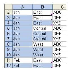
Result: You have a nice solid block of data with value in all of the rows for Region and Date, as shown in Fig. 971. This data is now suitable for sorting and filtering.
Summary: The steps above seem very convoluted. However, they can easily be mastered and carried out in less than a minute. They are the key to taking the results of a pivot table and creating a useful block of data for further analysis.
Images

Extra Tip
Problem: It is fairly cumbersome to navigate to the Edit – Paste Special – Value
Don’t blame me just because you are using these cool features all the time! Relax – there is an even faster way you can go. On the Standard toolbar, there is a Paste button. Next to the Paste button is a dropdown arrow, as shown in Fig. 111. From the arrow, you can choose to paste one of the six most common options: Paste Values, Paste Formats, No Border, Transpose, Paste Link, and Paste Special.


