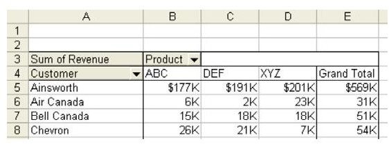
Problem: In a pivot table, a Data field will tend to inherit the numeric formatting assigned to the data in the original dataset. This may not always be correct. At a detail level, it might be appropriate to see invoice amounts in dollars and cents, as shown in Fig. 952. However, at a summary level, you might prefer to show numbers in thousands.
Strategy:
-
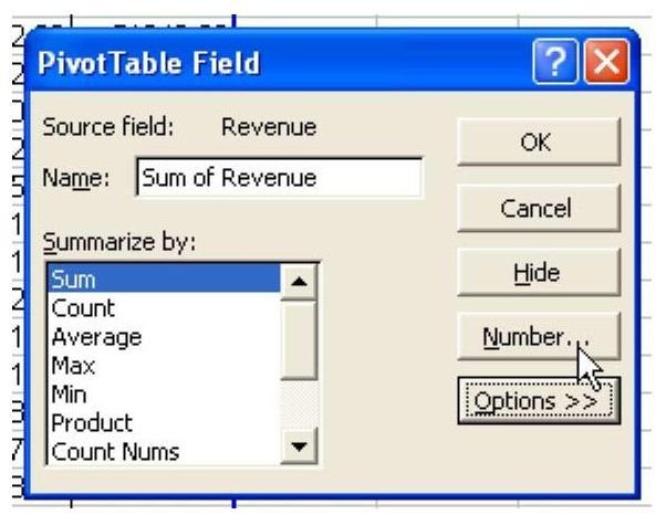
Assign a numeric format to the pivot field. Double-click the Sum of Revenue button to display the PivotTable Field dialog.
Advertisement -
Choose the Number… button, as shown in Fig. 953. Choosing the Number… button will bring up an abbreviated version of the Format Cells dialog with only the Number tab.
-
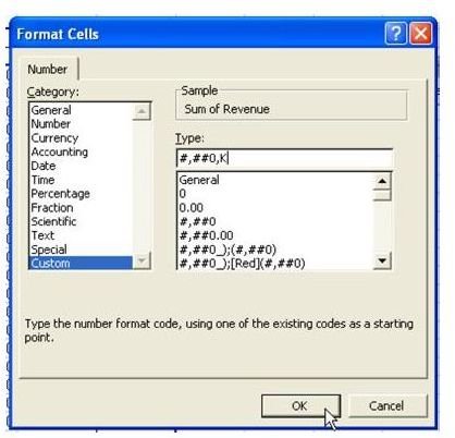
Choose an appropriate numeric format and select OK, as shown in Fig. 954.
Advertisement
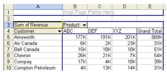
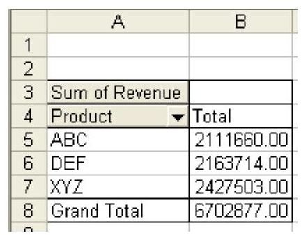
Result: As shown in Fig. 955, the Revenue field will now always show the selected format, no matter how the pivot table is changed.
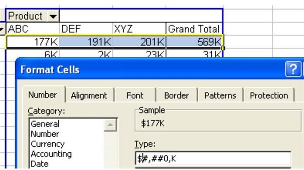
Gotcha: One of the conventions in formatting says that you should include a currency symbol on only the first and total rows of a dataset. There is not a good way to do this with a pivot table. Use the numeric formatting attached to the Product button to assign a currency format. Then, select the first row of cells and assign a new format using Ctrl+1 to display the Format Cells dialog, as shown in Fig. 956.
This will work initially, as shown in Fig. 957.
If you later resequence the pivot table, such as sorting by revenue, the special formatting will move into the pivot table instead of staying with the first row, as shown in Fig. 958.
Summary: You can control numeric formatting in a pivot table by using the PivotTable Field dialog.
Commands Discussed: PivotTable – Pivot Field – Number
Images