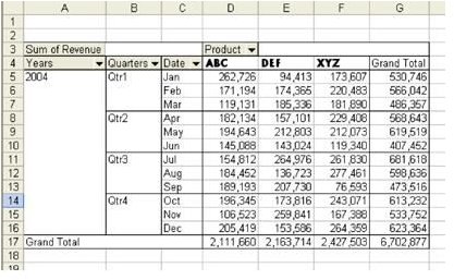
Problem: Due to the dynamic nature of pivot tables, it is fairly hard to format them. As shown in Fig. 943, you might want to format the headings in D4:F4 with a particular format because they are column headings. However, when you spin the pivot table to another shape, the formats will be lost.
Strategy:
Use one of the 22 built-in AutoFormats for pivot tables. Even if you don’t normally use AutoFormat in regular Excel, you should consider it in pivot tables.
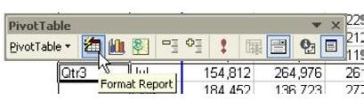
- Use the Format Report button on the PivotTable toolbar, as shown in Fig. 944.
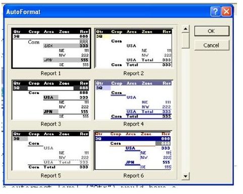
The AutoFormat dialog box initially shows six different report layouts. The examples show the formatting on a report with four fields in the Column area. As shown in Fig. 945, in Report 1, they are showing you that the innermost level (Zone) would have a normal black font on white. The next level (Area) would have a black font on a gray background. The outermost level (Qtr) would have a bold font.
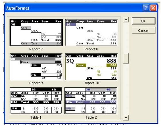
- As shown in Fig. 946, use the scroll bar to see the formats for Report 7 through Report 10 and Tables 1 through Table 2.
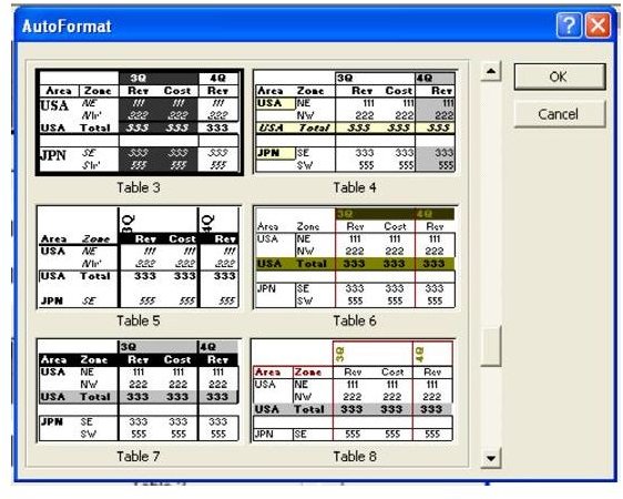
Fig. 947 shows Table 3 through Table 8.
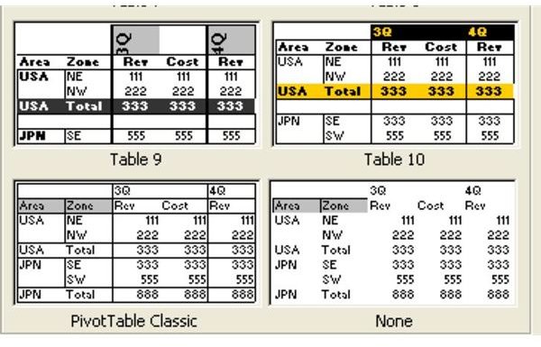
The last few options are Table 9, Table 10, PivotTable Classic, and None, as shown in Fig. 948.
- Choose one of the formats and select OK.
**
Result:
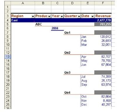
You can quickly apply a new look to the data. Fig. 949 shows Report 6.
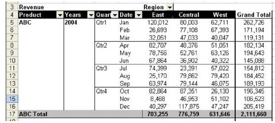
If you don’t like one look, choose the Format Report icon again and select a different look. Fig. 950 shows Table 7.
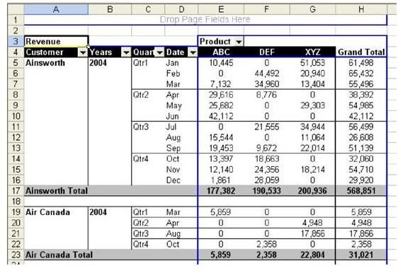
Even with these formats, you can still pivot the report as usual. Here, as shown in Fig. 951, the Product field moves up to the Column area, Region is removed, and Customer is added to the Row area.
Summary:
For years, I used pivot tables because of their ability to quickly produce summary reports. In recent versions of Excel, Microsoft has improved the pivot table by offering great looking ways to format the summary reports.
Commands Discussed:
PivotTable – Format Report
**
Images