Quick Take
Problem: You want to summarize data by Region, Product, and Customer. How can a two-dimensional report show three dimensions of data?
On this page
Strategy:
Several views of the data are possible. From the PivotTable Field List, drag the Region field and drop it in the Row area of the pivot table, to the left of the Customer field, as shown in Fig. 882.
Advertisement
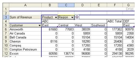
Another option is to drag the third measure to the Column area of the pivot table, as shown in Fig. 883.
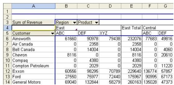
Even with this view, the report looks different if you move the Region field and drop it to the right of the Product field, as shown in Fig. 884.
Advertisement
Summary: You can use more than one field along either the row or column axis of the pivot table to produce more complex summaries.
Images
Advertisement