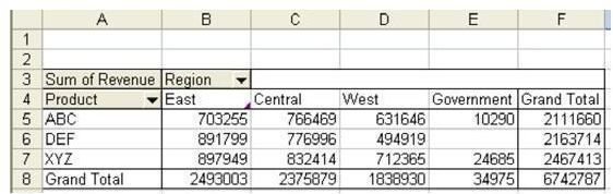
Problem: One number in the Pivot Table seems to be wrong. For example, maybe the Government region does not typically buy a certain product line from you, yet they are shown with that product in the report, as shown in Fig. 862.
Strategy:
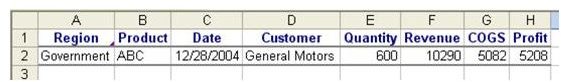
You can see the detail behind any number in a pivot table by double-clicking on the number. If the $10,290 in sales of product ABC to the government seems unusual, double-click cell E5. As shown in Fig. 863, a new worksheet is inserted with all of the records that make up the $10,290. In this case, it is just one record, which seems to have been coded to the wrong region.
**
Additional Information:
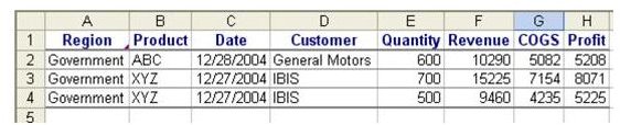
If you double-click on a number in the total row or total column, you will see all of the records that make up that number. Drilling down on E8 in the original pivot table will show the records that make up the $34,975, as shown in Fig. 864.
Gotcha:
Each drill down creates a new worksheet. The new worksheet is just a snapshot in time of what made up the original number. If you detect a wrong number in the drill down report, you need to go back to the original data to make the correction.
Summary:
Given the power to summarize data in a pivot table, you are likely to spot information that might point to a problem in the underlying data. With 50,000 rows of data, it is likely that someone miscoded the region on a few of the records. Until you look at a pivot table with a quick summary, it is hard to spot obvious problems like the one shown here. When you see a number that seems suspicious in a pivot table, double-click the number to drill down and see the records behind the data.
Commands Discussed:
Data – Pivot Table
**
Images