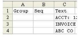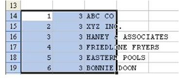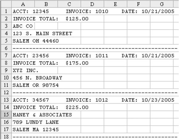
Problem: Sometime back, in the days of COBOL, a programmer was dealing with the constraints of the physical width of a page. The programmer built a report where each record actually took up five lines of the report, as shown in Fig. 815. You now want to analyze this data in Excel.
Strategy: Your goal is to get the data back into one row per record. This process is possible. The process involves adding two new columns, one called Group number and one called Sequence.
-
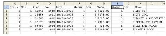
First, add a new Row 1. Insert two new columns A and B. Add headings as shown in Fig. 816 in A1:C1. The headings should be Group, Sequence, and Text.
Advertisement -
In column A, assign a Group number to each logical record.
One way to do this is to check to see if the first four characters of column C are
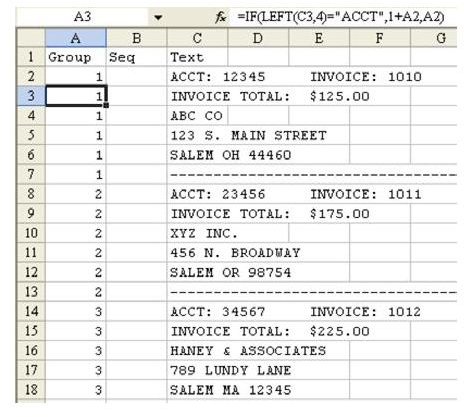
“ACCT”. If this is true, add one to the group number. In A2, enter the number 1.
In A3, enter the formula =IF(LE FT(C3,4)=“ACCT”,1+A2,A2). Copy it down to all
of the rows. This will neatly assign each logical group of records a group number, as shown in Fig. 817.
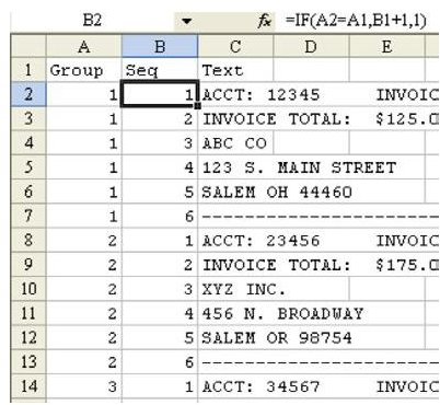
- Next, design a formula for a sequence number.
In cell B2, enter the formula =IF(A2=A1,B1+1,1). Copy this down. This formula will number each record in the group, as shown in Fig. 818. It should ensure that all of the Account numbers are on a Sequence 1 record.
-
This step is critical. Copy the formulas in columns A and B and paste them back, using Paste Special Values. This will ensure that you can safely sort the data.
-
Sort the data by the Sequence number in column B. Your data will look like Fig. 819.
Advertisement
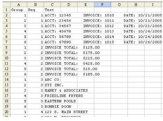
You have now managed to intelligently segregate the data so that all similar records are together. A contiguous range of C2:C7 contains all of the first rows from each record. All of the line 1 records have three fields that really should be parsed into three separate columns. You can easily do this with the Text to Columns Wizard.
-
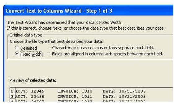
Select cells C2:C7. From the menu, select Data – Text to Columns. Select Fixed Width and Next, as shown in Fig. 820.
Advertisement -
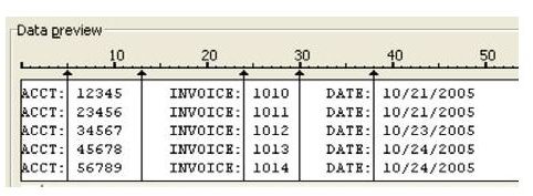
Excel should properly guess where your columns are, as shown in Fig. 821. Click Next.
-
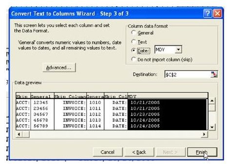
Choose the heading for each column and define a data format. You don’t really need the word ACCT each time, so choose to Skip the first, third, and fifth fields. Make the sixth field a date. When your information looks like Fig. 822, choose Finish.
Advertisement -
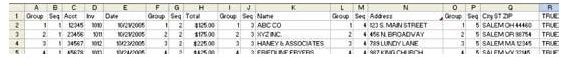
You will have data in three columns of Group 1. As shown in Fig. 823, change the heading in C1 to be Acct, the heading in D1 to be Inv, and the heading in E1 to be Date.
-
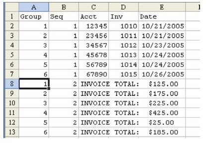
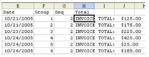
Next, select A8:C13. Cut and paste in F2. Add headings in F1:H1 of Group, Seq, and Total, as shown in Fig. 824.
Advertisement -
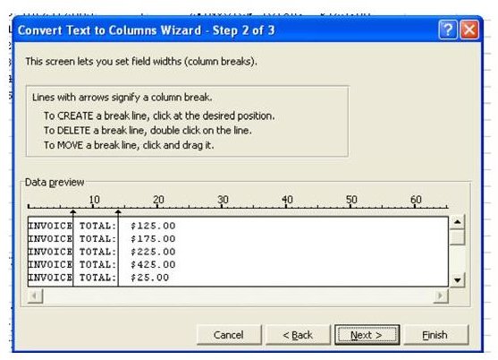
Select H2:H6 and choose Data – Text to Columns. In Step 1, select Fixed Width and choose Next. In Step 2, Excel offers to split your data into three fields. There is no need to have one column for the word Invoice and another column for the word Total. As shown in Fig. 825, double-click the line between Invoice and Total to delete the line.
-
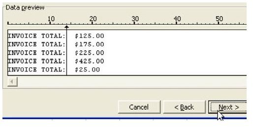
After double-clicking the first line, it is deleted. Choose Next, as shown in Fig. 826.
Advertisement -
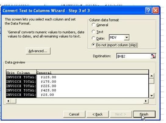
In Step 3, choose to skip the field with “Invoice Total” and choose Finish, as shown in Fig. 827.
-
Select the Group 3 records, as shown in Fig. 828.
Advertisement -
Copy them to I2. The headings in I1:K1 are Group, Seq, and Name, as shown in Fig. 829.
-
Select the Group 4 records. Cut and paste in L2.
Advertisement -
Select the Group 5 records. Cut and paste in O2.
-
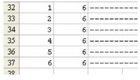
As shown in Fig. 830, the Group 6 records have no data – they are just dashed lines. You can delete these rows.
Advertisement
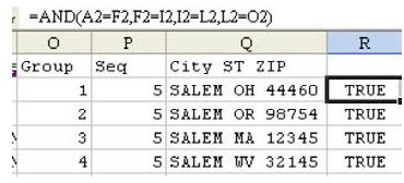
You now have all the fields, one line per record. You also have the words Group and Sequence taking up about five columns each. Before you delete the Group and Sequence columns, let’s make sure that everything worked correctly. The Group numbers in columns A, F, I, L, and O should all match.
- As shown in Fig. 831, in a blank column at the end, enter a large AND function as shown below. Copy this formula down to all rows:
=AND(A2=F2,F2=I2,I2=L2,L2=O2)
-
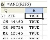
A value of True means that you have successfully put all of the Group 1 records back together. To test if all of the rows have True, enter the formula =AND(R2:R99) in cell R1. As shown in Fig. 832, if this formula is True, then you’ve crosschecked that all of the rows match up.
-
At this point, you can delete the columns that you don’t need. As shown in Fig. 833, delete columns R, P, O, M, L, J, I, G, F, B, and A.
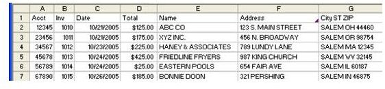
Result: You now have a sortable, filterable, and reportable version of the original dataset. Each record consists of one row in Excel, as shown in Fig. 834.
Summary: This process is convoluted. However, if you are presented with data as shown in the original example, the only way to quickly add up figures or to produce a report is to follow steps similar to the ones shown in this topic.
Commands Discussed: Data – Text to Columns
Functions Discussed: =IF(); =AND(); =LEFT()
Images