Problem: You want to buy a car. You want to compare eight price points and four loan terms to calculate the monthly payment amount.
Strategy:
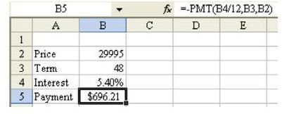
There are two methods. The cool method is to use a data table. As shown in Fig. 764, set up the worksheet as follows:
-
Enter one price in cell B2.
-
Enter one term in cell B3.
Advertisement
- Enter the current annual interest rate in B4.
- In cell B5, enter a formula to calculate a monthly payment:
=–PMT(B4/12,B3,B2)
Cell B5 is going to be the magic corner cell of your data table.
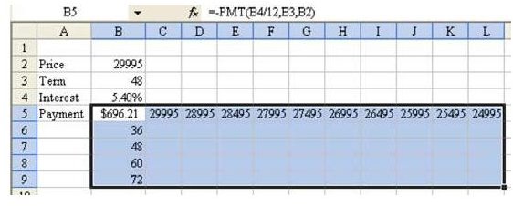
- In cells B6:B9, enter the four possible terms that you would like to compare. In cells C5:L5, enter the possible prices that you hope to negotiate to, as shown in Fig. 765.
- Select the rectangular range of B5:L9. As shown in Fig. 765, the upper left corner of this range contains the formula to calculate your monthly payment.
-
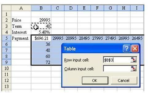
From the menu, select Data – Table. Excel will ask you to specify a row input cell. In other words, Excel will take each cell in the top row of the table and substitute it for this cell. Because these cells contain prices, choose cell B2 as the row input cell, as shown in Fig. 766.
-
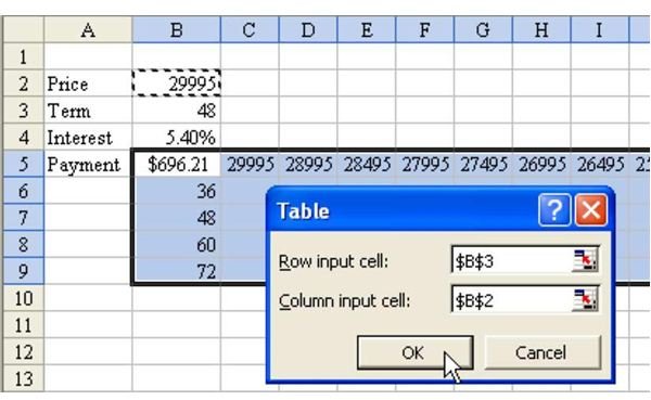
Next, Excel wants to know where the cells in the first column should be used. Because B6:B9 contains terms, specify cell B3, as shown in Fig. 767. Choose OK.
Advertisement
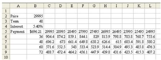
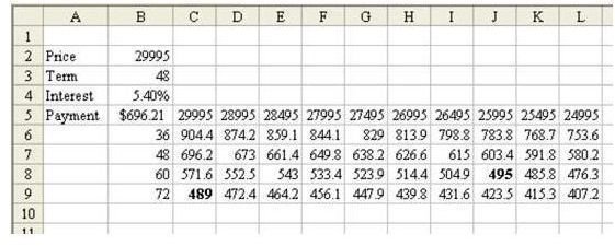
Excel enters an array formula for you. You can see the monthly prices for many combinations of terms and price points, as shown in Fig. 768.
If you are looking for a monthly payment of $495, you will have to either negotiate down to a price of $25,995 with a 60-month loan, or choose a 72-month loan, as shown in Fig. 769.
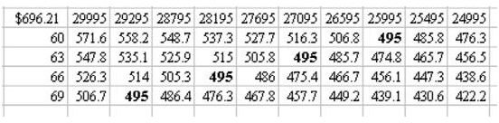
The formulas in the table are live. As shown in Fig. 770, you can re-enter new values in the first column and row of the table in order to zoom in on possible scenarios.
**
Additional information:
You can also change the formula in B5 and the table will update.
Summary:
The Data Table command is a powerful command for comparing several what-if scenarios.
Commands Discussed:
Data – Table
Strategy:
**
There are two methods. The cool method is to use a data table. As shown in Fig. 764, set up the worksheet as follows:
-
Enter one price in cell B2.
Advertisement -
Enter one term in cell B3.
-
Enter the current annual interest rate in B4.
Advertisement -
In cell B5, enter a formula to calculate a monthly payment:
=–PMT(B4/12,B3,B2)
Cell B5 is going to be the magic corner cell of your data table.
-
In cells B6:B9, enter the four possible terms that you would like to compare. In cells C5:L5, enter the possible prices that you hope to negotiate to, as shown in Fig. 765.
-
Select the rectangular range of B5:L9. As shown in Fig. 765, the upper left corner of this range contains the formula to calculate your monthly payment.
-
From the menu, select Data – Table. Excel will ask you to specify a row input cell. In other words, Excel will take each cell in the top row of the table and substitute it for this cell. Because these cells contain prices, choose cell B2 as the row input cell, as shown in Fig. 766.
-
Next, Excel wants to know where the cells in the first column should be used. Because B6:B9 contains terms, specify cell B3, as shown in Fig. 767. Choose OK.
Excel enters an array formula for you. You can see the monthly prices for many combinations of terms and price points, as shown in Fig. 768.
If you are looking for a monthly payment of $495, you will have to either negotiate down to a price of $25,995 with a 60-month loan, or choose a 72-month loan, as shown in Fig. 769.
The formulas in the table are live. As shown in Fig. 770, you can re-enter new values in the first column and row of the table in order to zoom in on possible scenarios.
**
Additional information:
You can also change the formula in B5 and the table will update.
Summary:
The Data Table command is a powerful command for comparing several what-if scenarios.
Commands Discussed:
Data – Table
**
Images