Problem: Your manager wants you to add a blank line between sections of the subtotal report. This is a fairly standard request. Quite simply, data looks better when it is formatted this way.
Strategy: This is really hard. There is no built-in way to do this. I’ve tried many methods. I picked the three best methods to explain here.
Method 1:
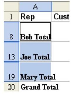
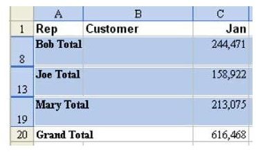
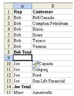
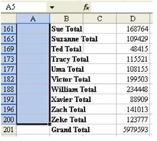
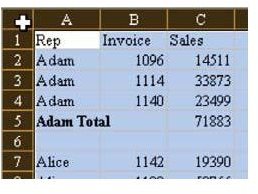
1) To do this easily, follow the steps in the preceding “bold pink Tahoma font” chapter. Add subtotals, collapse to level 2, select column A between the headings and grand total, Edit – Go To – Special– Visible Cells Only. You will then have selected just the subtotal rows, as shown in Fig. 721.
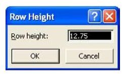
2) From the menu, select Format – Row – Height. Depending on your font, the row height will probably be between 12 and 14. The height shown here in Fig. 722 is 12.75.
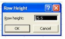
3) Mentally multiply by 2 and type 25.5 as the new height, as shown in Fig. 723.
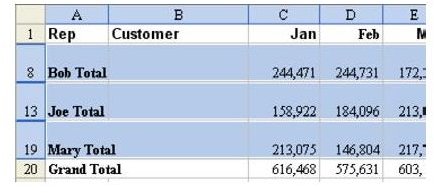
This creates a fairly ugly intermediate result, as shown in Fig. 724.
4) Select everything from the first subtotal to the last subtotal again, this time selecting all of the columns in the dataset. As shown in Fig. 725, use Edit – Go To – Special – Visible Cells Only.
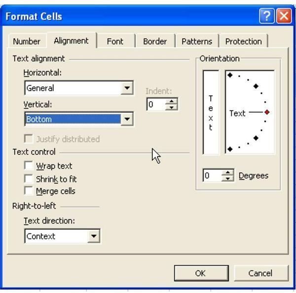
5) Press Ctrl+1 on the keyboard to display the Format Cells dialog. Select the Alignment tab. By default, you will see that the Text Alignment – Vertical is set to Bottom, as shown in Fig. 726.
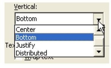
6) Choose the Vertical dropdown arrow. As shown in Fig. 727, you will appear to have choices for Center, Bottom, Justify, or Distributed.
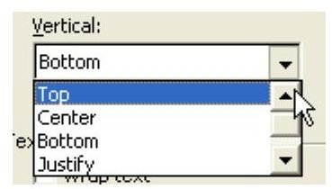
7) Use the up scrollbar to display the other choice: Top, as shown in Fig. 728.
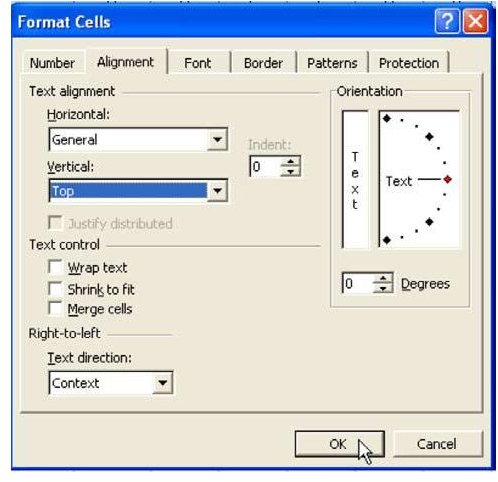
8) Select Top and choose OK, as shown in Fig. 729.
As shown in Fig. 730, the intermediate result looks only slightly better.
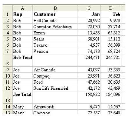
9) Choose the Group & Outline button #3 to display the detail rows again, as shown in Fig. 731.
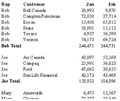
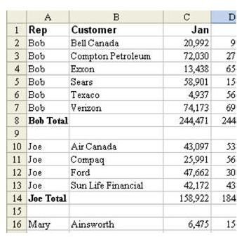
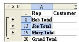
Although you can see that there is no blank row after the subtotals in rows 8 and 13, when you print the report for your manager, it will appear to have a blank row, as shown in Fig. 732.
10) From the menu, select Insert – Row. You will have inserted 50 rows at the appropriate spots, as shown in Fig. 747.
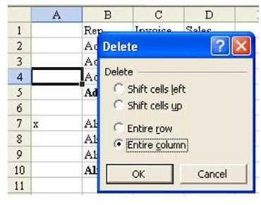
11) You can now delete the temporary column A. Select any cell in column A and choose Edit – Delete – Entire Column, as shown in Fig. 748.
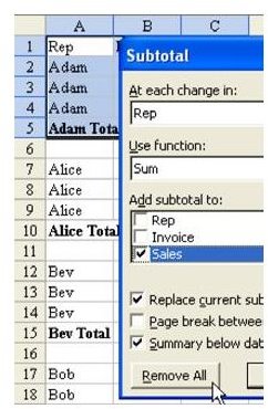
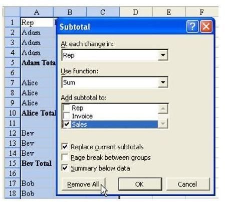
Gotcha: In order to delete all of the subtotals, you will have to select the entire range before calling the Data Subtotals command. One fast way to do this is to click on the blank gray box above and to the left of cell A1. This box will select all cells in the worksheet, as shown in Fig. 751.
Now when you choose Data – Subtotals, you will find that Excel has selected all of the subtotals. Click Remove All to remove the subtotals, as shown in Fig. 752.
There are three methods for inserting a blank row between each group of subtotals. You can see that none of the three methods seem very appealing, which means that this fairly common request is fairly hard to do. However, with practice, you will find that the third method can be accomplished quickly.
Once the blank rows are in, you may have a difficult time getting rid of the subtotals. As shown in Fig. 750, if you select cell A2 and choose Data – Subtotals – Remove All, Excel will only delete the first subtotal. As shown in Fig. 749, you will have quickly added the blank rows requested by the manager. The third method is to attempt to make method 2 faster. This is particularly important if you have 50 reps. Follow these steps.
1) Add subtotals. Collapse to Group & Outline level 2, as shown in Fig. 736.
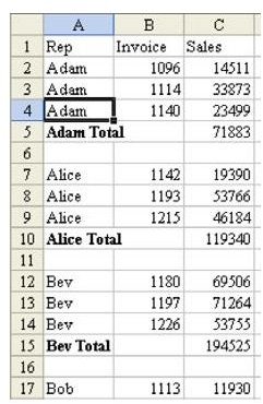
2) Insert a new temporary blank column A to the left of the current column A, as shown in Fig. 737. To do this, select any cell in column A and choose Insert – Column
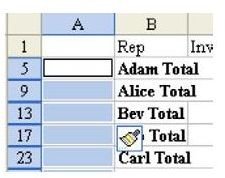
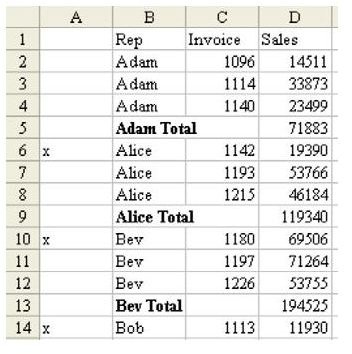
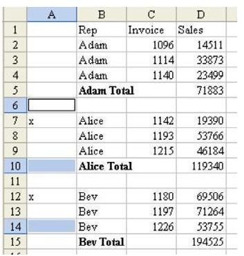
3) The goal is to enter an x next to each subtotal in column A. With the mouse, drag from A5 down to the last row with a subtotal in A, as shown in Fig. 738.
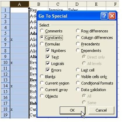
4) Select Edit – Go To – Special – Visible Cells Only, as shown in Fig. 739.
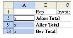
5) Type an x and hit Ctrl+Enter to place the x in all selected cells, as shown in Fig. 740.
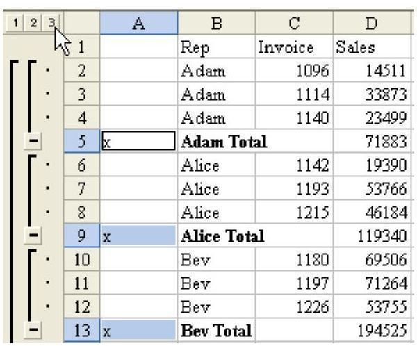
6) As shown in Fig. 741, choose the #3 Group & Outline button to unhide the detail rows.
7) The next step is to move all of the “x” values down one cell. It is tempting to hit Ctrl+X to perform a Cut, but this will not work on non-adjacent cells, as shown in Fig. 742.
8) Select from A5 through the last x in column A, as shown in Fig. 743.
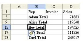
9) Use Edit – Cut or Ctrl+X to cut the cells. Move down one cell to A6. Hit Ctrl+V or Edit – Paste to place the “x” cells on the first row of each subtotal group, as shown in Fig. 744.
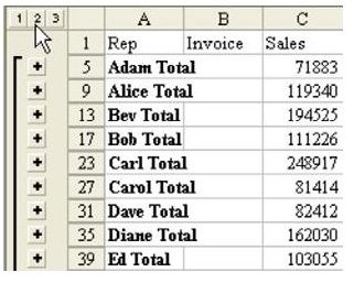
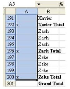
10) You want to select all of the rows with an x in column A. Select the entire column by using the mouse on the gray “A” at the top of the column. Choose Edit – Go To – Special – Constants, as shown in Fig. 745.
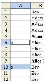
You will have now selected just the first cell of each group, as shown in Fig. 746.
The second method is to use old-fashioned, brute force. Insert a blank row between each group method.
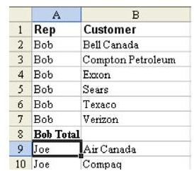
1) As shown in Fig. 733, go to cell A9.
2) Hold down Alt while you press I and then R. As shown in Fig. 734, this will insert a row above the current cell, using the Insert – Row command.
3) Go to cell A15 and insert another row. This method is easy when you have three sales reps as shown here in Fig. 735, but very tedious when you have 50 sales reps.
will not work if you have to send the dataset to the manager via e-mail. The manager may be smart enough to want to stop at each subtotal using the End key, and this will not work with the double height rows.The first method is to try to fool the manager by making the total rows be double-height, with the totals vertically aligned to the top. This method may work if you are printing the report to give to the manager. It will give the appearance that a blank row has been inserted.
Images