In this Microsoft Excel tutorial, we’ll explain how the TRANSPOSE function can be used to transform rows of data into columns.
Turning Rows into Columns with TRANSPOSE
Have you ever spent hours creating a list or table in Excel and then wished you had organized the data in columns rather than rows (or vice versa)? Rather than start all over again, you can use the TRANSPOSE function to your data from rows to columns or columns to rows.
Syntax of the TRANSPOSE Function
The syntax for a basic formula using the TRANSPOSE function is
{=TRANSPOSE(array)}
where the array argument consists of the group of cells that you want to convert from row data to column data (or the other way around).
One thing that is important to note in the syntax of this function is the placement of the braces. These braces tell Excel that your answer should be another array rather than just a single cell. If you forget to include them, you’ll either get an error or only one cell from the original list or table will be transposed. However, these braces are added after the rest of the formula is composed, as we will show in the example in the next section.
Example of the TRANSPOSE Function
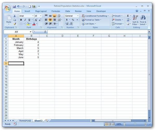
To illustrate the TRANSPOSE function, we’ll use a simple table that lists several months and the number of family birthdays in each month. See the screenshot below. (Click any image for a larger view.)
In this example, we have a table that is 7 rows by 2 columns, and we would like to transform it into one that is 2 rows by 7 columns.
Step 1: First, we need to select the cells in which we want the transformed cells to appear. In this case, we need to select a group of cells on the worksheet that is 2 rows high by 7 columns long.
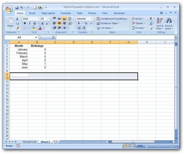
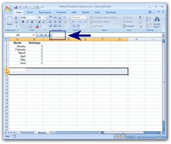
Step 2: With these cells selected, click on the formula bar in the area shown in the screenshot below.
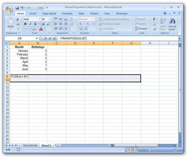
Step 3: Type in the formula containing the TRANSPOSE function. Since the initial table that we want to transpose is in cells A1 through B7, our array is A1:B7. Even though we will need the braces eventually, don’t worry about that just yet. We’ll explain that in a moment. For now, type in the main part of the TRANSPOSE function as shown below, but don’t hit the Enter key yet.
=TRANSPOSE(A1:B7)
Step 4: Once the formula is typed in, hit Ctrl + Shift + Enter instead of just Enter. This will place the braces around the formula and evaluate it in the worksheet as shown below.
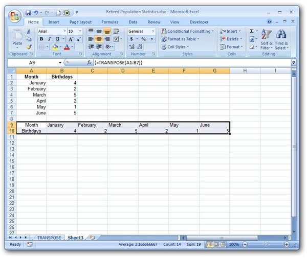
Note that the TRANSPOSE function only copies the data from the cells in the initial array. If you had applied any special formatting to those cells, you will need to do that again.
Additional Resources: If you’re looking for other Excel tutorials, be sure to browse through the ever-growing library of users guides found here on Bright Hub’s Windows Channel, including the collection covering charts and graphs .