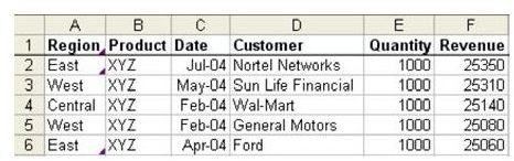
Problem: You have 10,000 records, as shown in Fig. 641; you need to be able to quickly find records that match a criterion, such as all East ABC records.
See all Microsoft Excel tips
Strategy: Use the AutoFilter feature.
-
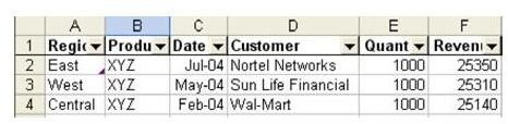
Make sure your data has a heading row. From the menu, select Data – Filter – AutoFilter. You will have a dropdown on each heading, as shown in Fig. 642.
-
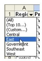
As shown in Fig. 643, use the dropdown to select East from the region dropdown.
Advertisement -
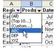
As shown in Fig. 644, select ABC from the Product dropdown.
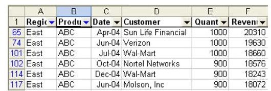
Result: You will see only sales of product ABC in the East region, as shown in Fig. 645. All of the other rows will be hidden.
Caution: To copy just the filtered records, you will have to use Edit – Go To – Special – Visible Cells Only to select only the visible cells on the sheet.
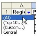
Additional Information: There are three special choices at the top of each column.
-
Use (All) to “cancel” a filter on one column, as shown in Fig. 646.
-
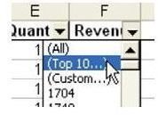
As shown in Fig. 647, use Top 10… to see the top N records or the top n percent of the records.
Advertisement -
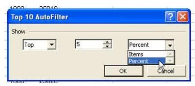
After you select Top 10, the Top 10 AutoFilter dialog appears, as shown in Fig. 648. You can choose if you want the top 10 percent or the top 10 items, and also change the “10” to “5” or to any other number. This can also be used to show the bottom 10 records.
-
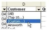
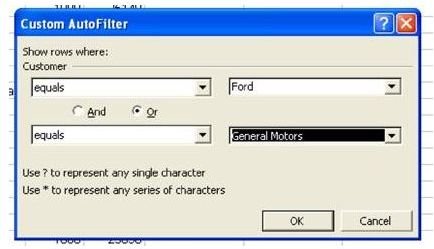
As shown in Fig. 649, use Custom to build a criteria joined by AND or OR.
Advertisement -
In the Custom AutoFilter dialog box, you can choose two values and specify whether they should be joined by AND or OR, as shown in Fig. 650.
-
To remove the AutoFilter dropdowns and show all records, go to the Data menu again and re-select AutoFilter. This will toggle the AutoFilter off.
Advertisement
Summary: Use Data – Filter – AutoFilter to have Excel show you data matching certain criteria in a column.
Commands Discussed: Data – Filter – AutoFilter
See all Microsoft Excel tips
Images