How to Make a Line Graph in Excel: Step by Step Tutorial

Getting Started

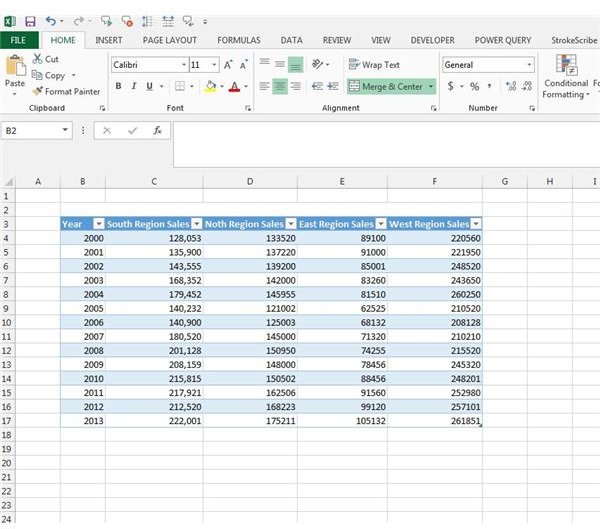
Before you can create a line graph, you need to enter data. The manner in which you organize your data is important. The more organized the data, the easier time you will have creating your line graph. List your data categories, such as year, sales or items along the top of your chart. Enter the data in the appropriate columns.

For our example, I have populated an Excel spreadsheet with several columns. One represents a year, while the others represent sales at a fictional store by regional area (Figure 1). We want to create a line graph depicting this data.

Line Graphs Made Easy

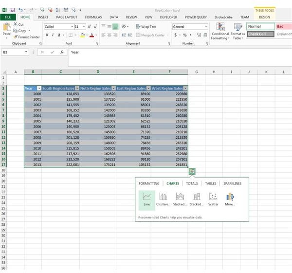
One of Excel 2013’s best new features is the ability to grab a section of data and instantly turn it into a graphical depiction using the Quick Analysis button. In our example, I simply highlighted the data I wanted in the graph, which causes a small button to pop up at the bottom right of the selected cells. If you click on it, the Quick Analysis menu will appear (Figure 2). From here, you can click on Chart and then on Line.

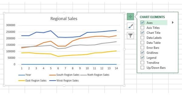
Excel will create a chart based on the data you selected and insert it into your spreadsheet (Figure 3).

Images

Customizing Your Chart

The Quick Analysis tool is great for getting a quick chart on your sheet. Maybe you want to tweak some things. Let’s look at some of the customization options you have in Excel 2013.

Chart Title
To change the chart title, double-click the Chart Title placeholder text.

Modify Elements Are Displayed
You can easily change which chart elements are displayed by clicking on the chart and then clicking on the “+” icon. From here, you can select or de-select items such as axes, titles, trend lines, data points and a data table.

Change the Appearance
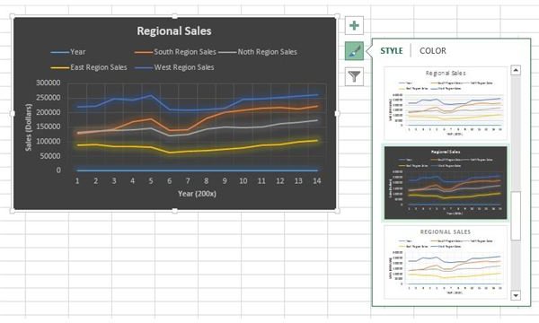
In order to change the color scheme, click on your chart and then click the Paintbrush icon. From here, you can choose a different style and color scheme (Figure 5).

Filter What Is Displayed
You can filter what is displayed using the filter icon. Click your chart and then click the filter button. Simply select or de-select which items you wish to display on the chart.

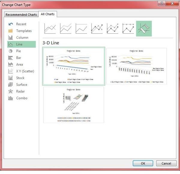
Change Chart Type
If you don’t like the overall layout of your chart, you can click on the chart and then click on Chart Tools -> Design -> Change Chart Type. From here, you have the option of changing the overall look of your chart. In Figure 6, you can see I have selected All Charts and then the Line -> 3D Chart type.

The Chart Tools Ribbon

Note that instead of interacting directly with your chart, you can also use the Chart Tools ribbon bar to view all of your options on one menu. Color, chart elements and chart style can all be modified from the ribbon interface.

I hope that you have learned how to create line graphs effectively in Excel. Don’t be afraid to experiment with the variety of options you have when creating charts in Excel.