Even though most people associate Excel with numbers and databases, the software also has a number of drawing tools to help with data presentation.
Problem: You have a large spreadsheet with many calculations. Results from section 1 are carried forward to cells on section 2. It would help to graphically illustrate that one cell flows to the calculation of another.
Click any figure for a larger view of that image.
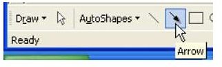
Strategy: Use the Drawing toolbar, as shown in Fig. 1330. If this is not visible at the bottom of your worksheet, then use View – Toolbars – Drawing. The toolbar typically appears at the bottom of the screen. Use the Arrow tool shown here.
-
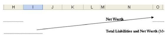
Click in the origin cell and drag to the final cell. When you release the mouse button, an arrow will appear, pointing from the first cell to the end cell, as shown in Fig. 1331.
Advertisement -
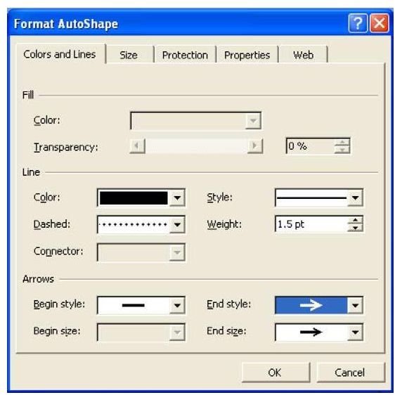
Use your mouse pointer to click on the line. Selection handles will appear. Right click and choose Format Drawing Object.
-
As shown in Fig. 1332, in the Format dialog you can customize line width, arrow style, color, etc.
Advertisement
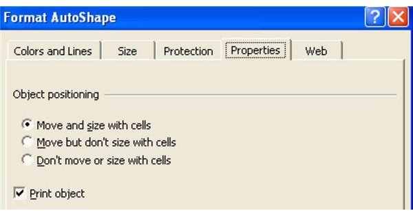
Note: The Properties tab of the dialog controls whether the arrow prints or not. Perhaps the most important property is the checkbox for Move and Size with Cells, as shown in Fig. 1333. If you leave this unchecked and insert rows between the origin and final cell, the arrow does not resize to keep pointing at the final cell.
Summary: Create a variety of arrows to help graphically illustrate the flow of your spreadsheet.
Commands Discussed: View – Toolbars
Images
References and Additional Resources
If you’re looking for more tips and tutorials, check out 91 Tips for Calculating With Microsoft Excel . This collection of easy-to-follow guides shows how to customize charts and graphs, different ways to make complex spreadsheets easier to update, and even how to play games like Craps in Excel.
Other Resources:
Microsoft Excel Official Site, https://office.microsoft.com/en-us/excel/
Bill Jelen, Microsoft Excel 2010 In Depth, Available from Amazon.com .