There are quite a few lookup and reference functions in Microsoft Excel, several of which seem to do the exact same thing. When should you use which?
Overview
Within Excel, there is a group of functions that have been specifically designed to lookup and reference information in a spreadsheet. These tools are especially useful if you’re trying to create some type of form or other interactive object within the constraints of Excel. The trouble is that many of these functions seem to perform the exact same duties – so when should you use each one?
Which Function to Use?
One of the most general items in this list is the aptly named LOOKUP function. However, names can be deceiving. While this function can be quite useful in
some cases (for a specific example, see this more in-depth tutorial on Excel’s LOOKUP function ), it has a few limitations that make it impossible to use in every situation.
Basically, the LOOKUP function will search the first row or column of an array and return a value from the last row or column of that same array. Alternatively, you can specify a single row or column as the lookup vector and another as the result vector, but this requires that your data be sorted in a very specific manner. To that end, it’s often more advantageous to use the more detailed HLOOKUP and VLOOKUP functions.
The HLOOKUP and VLOOKUP functions are virtually identical in construction with the only real difference being HLOOKUP is used when data is arranged in rows and VLOOKUP when arranged in columns. (See this article on HLOOKUP and VLOOKUP functions for more details.) One nice thing about these two functions is that you’re not restricted to just looking for results in the last row or column of the array. Instead, you can designate exactly which row or column from which to return a result. Additionally, when using the “exact match” option, you don’t have to worry about sorting at all.
An even more specific function that allows you to lookup data in a table is the INDEX function. When using this function, however, you do need to specify an exact row and column in the array you are querying. A more detailed example of this process can be found in Microsoft Excel’s INDEX Function .
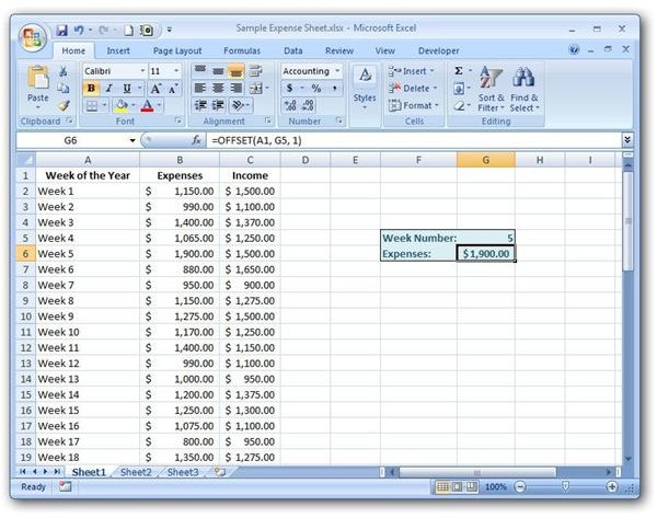
A similar tool is Excel’s OFFSET function. Instead of specifying an exact row and column in the array to query, the OFFSET function chooses a row and column from an initial reference point that is defined in the function. To get a better idea about how this function works, take a look at this example involving the OFFSET function .
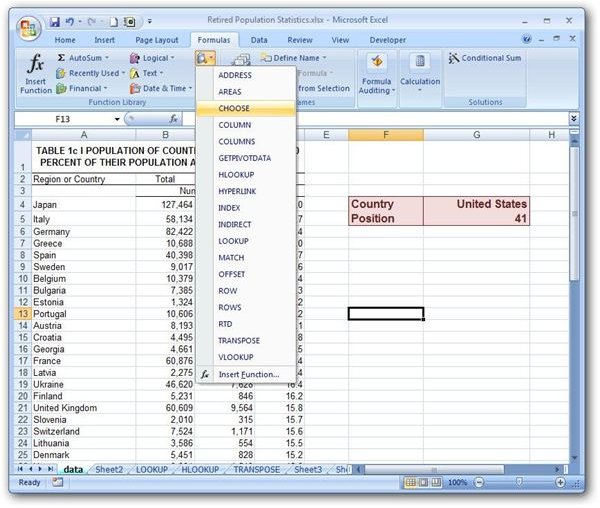
If you’re more concerned with retrieving the position of an item in a list or table than you are with returning a value associated with that item, it’s probably easier to use the MATCH function. (See Microsoft Excel’s MATCH Function .) With this function, you can specify a row or column in an array and determine the ranking of any item in that list.
Additional Resources: For more Excel tips and tricks, have a look at some of the other articles in Bright Hub’s collection of Excel user guides. Learn about chart and graph design , how to create a dependant drop down list , and other useful tricks. More items are being added on a regular basis, so keep checking back.


