How to Create a Depreciation Schedule in Excel

Create a Depreciation Schedule in Excel from Scratch

This tutorial uses straight line depreciation for simplicity. However, modifying the straight line formula with the formula that you want to use, such as Double Declining Balance, is all that is necessary to change the depreciation method.

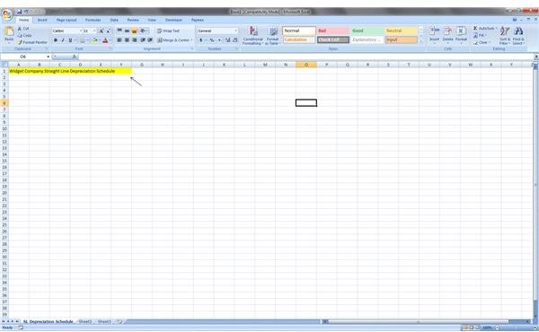
1. Open Microsoft Excel and rename the first tab to Depreciation Schedule. If several schedules are preferred for comparison sake, name the tab to something like “SL Depreciation Schedule.” Other tabs can be created for Double Declining Balance, etc.

2. Place a title, such as “ Straight Line Depreciation Schedule” in row one.

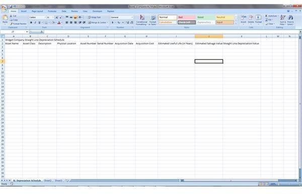
3. Name the columns as so:

• Column A Row Two = Asset Name
• Column B Row Two = Asset Class
• Column C Row Two = Asset Description
• Column D Row Two = Physical Location
• Column E Row Two = Asset Number
• Column F Row Two = Serial Number
• Column G Row Two = Acquisition Date
• Column H Row Two = Acquisition Cost
• Column I Row Two = Estimated Useful Life (In Years)
• Column J Row Two = Estimated Salvage Value
• Column K Row Two = Straight Line Depreciation Value

Format the Depreciation Schedule

The bones of the schedule are complete. Now it’s time to format the document.

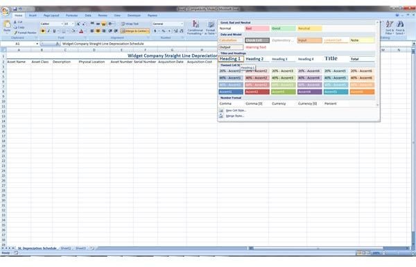
1. Highlight the title and all the columns through column K in row one. Click on “Merge & Center.”
2. Click on the Quick Formatting Bar and choose the “Heading 1” option.
3. Highlight the cells in row two from Column A to Column K. Right click to bring up the short menu. Click on the “Format Cells” option. A dialog box will open. Click on the “Alignment” tab and choose the checkbox for “wrap text.” Choose the “center” option from the main formatting menu to center the text in these cells.
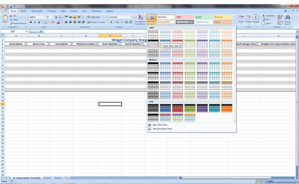
4. Choose to bold the titles, change the color of the text, and alternate the colors of the rows however you please. One quick way to format a table in Excel is to use the “Format as Table” option in the formatting menu. Make sure to select the “My table has headers” option.
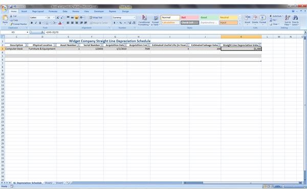
5. Start filling in the data from Column A to Column J.
6. Enter the straight line formula in Column K. For example, the formula for row 3 would be: =(H3-J3)/I3.

Tips:

1. Cells can be formatted further as currency, text, date, etc. by right clicking the cell to display the quick menu and selecting “Format Cells.”
2. When highlighting cells across columns be sure to not click the row header (ie the row number 2) for example. This will highlight all the columns across the entire spreadsheet and could cause printing problems if a format such as “borders” were to be applied.
3. If the “Format as Table” option is used and the check box “My table has headers” is appropriately checked, then drop down arrows appear in the cells for row 2. The arrows allow for sorting the rows.

That’s all there is to it. The depreciation schedule is now ready to use as a tool for bookkeeping or tax purposes.

Screenshots

Create a Depreciation Schedule in Excel Using a Template

Learning to use a tool from scratch is important for independence and skill growth. However, there is an easier method for creating a depreciation schedule in Microsoft Excel using templates.

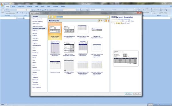
1. Open Microsoft Excel and click the new button.
2. In the search bar, located at the top of the dialog box, click on schedules and search for “Depreciation.” Notice that there are several templates to choose from.
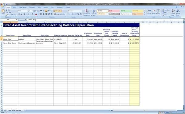
3. Select the desired template.
4. Start entering data.

That’s all there is to it. Be sure to save the new document to your computer. When working with large lists, it is a good idea to save the work intermittently.

Screenshots