Moving averages have long been used to define trends in data from various sources, from weather and climate to investment markets. Different methods for computing moving averages yield slightly different results and benefits, making certain averages particularly well suited for investment analysis.
Exponentially Weighted Moving Average
We covered simple moving averages in an earlier article, where we saw that moving averages smooth out the fluctuations from each individual datum so that we can better see trends over desired intervals. Exponentially weighted, or exponential moving averages (EMA) follow the same idea and serve the same purpose, while giving us two additional benefits missing in other averages.
Computation & Benefits
We explored the advantage of a weighted moving average over a simple moving average; that advantage is the increased contribution, or influence, from the most recent data. We change the amount of influence by changing the length of the average interval, which in turn changes the weighting factors. We showed a 5-day weighted moving average that uses the values 5, 4, 3, 2, and 1 as the weighting factors. Thus, the most recent datum has 5 times the influence of the oldest datum. A 10-day weighted moving average would give the most recent datum 10 times the influence of the oldest datum.
The exponential moving average (EMA) provides the same benefit by weighting the most recent datum more heavily than all preceding data. However, the weighting factor is constant, but is still derived from the length of the averaging interval. The EMA weighting factor is designated by the lowercase Greek α (alpha) and is computed as:
α = 2 / (N + 1)
where “N” is the number of days in the averaging interval. Using our 5-day intervals from our previous examples, α would be:
α = 2 / (5 + 1) = 2 / 6 = 1 / 3 = 0.33
Every computation of the present 5-day EMA value will use 0.33 as the weighting factor. So how is this a benefit over our previous methods? It isn’t! This feature of EMA, by itself, provides no benefit because it weights each datum identically; which means that there’s no “weighting” at all. It’s the next feature of EMAs that is the necessary piece to provide the weighting…and the significant difference between EMAs and other average computation methods.
We’ve only shown how to compute α, the weighting factor, or coefficient, piece of the exponential moving average computation. The computation of each new EMA value is:
EMAN = ((DatumN - EMAN-1) * (α)) + EMAN-1
or, today’s EMA value, EMAN, is the weighting factor α times the difference between today’s datum (DatumN) and the previous day’s EMA value (EMAN-1). If we expand the above equation we get:
EMAN = (α * DatumN) - (α * EMAN-1) + EMAN-1
= (α * DatumN) + ((1-α) * EMAN-1)
The second equation above is the standard definition for computing EMA. If we use our 5-day interval α that we computed above as 0.33, our EMA equation becomes:
EMAN = (0.33 * DatumN) + (0.67 * EMAN-1)
Notice that the present day’s EMA value contains a portion of the previous day’s EMA value. This is what makes EMAs different, and more valuable, than our prior moving average examples. In our prior examples, the oldest datum dropped out of the computation as it got replaced by the newest datum. After the number of days in the computation interval a datum no longer contributed to the average. Because each day’s EMA value is determined by the present day’s datum and the previous day’s EMA value, all of the previous data is in each day’s EMA value…just to a lesser and lesser degree. Let’s look at the above equation again, focusing on the (0.67 * EMAN-1 factor. This means that the previous day’s EMA value contributed 67% of today’s EMA value. The EMAN-1 value was computed as:
EMAN-1 = (0.33 * DatumN-1 + (0.67 * EMAN-2)
Let’s substitute EMAN-1 from the above equation into the EMAN equation:
EMAN = (0.33 * DatumN + (0.67 * (0.33 * DatumN-1 + (0.67 * EMAN-2))
= 0.33 * DatumN + (0.67 * 0.33 * DatumN-1 + (0.67 * 0.67 * EMAN-2))
= (0.33 * DatumN) + (0.22 * DatumN-1) + (0.45 * EMAN-2)
Today’s EMA value (EMAN) consists of 33% of today’s datum value, 22% of the previous day’s datum, and 45% of the second previous day’s EMA value (EMAN-2). The EMAN-2 value contains all of the previous data up to that day’s.This is the power and the value of EMAs: all previous data remains in the computation for every successive value, just to an exponentially decreasing amount. Hence the name exponentially weighted moving average.
Comparing EMA to SMA and WMA
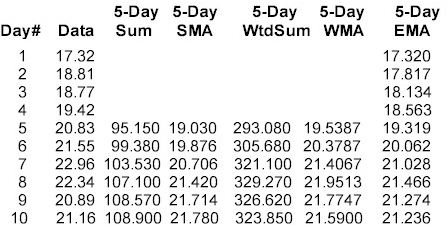
Let’s use the same 10 data values from our simple and weighted moving average examinations to compute our EMA values. Here we see another difference from other moving averages. Because all previous data remains in each EMA computation, the EMA value isn’t valid until you have computed the number of EMA values equal to the interval length. In our 5-day example, the EMA value won’t be valid, or stabilized, until the 5th day. We’ll use the first day’s data as the starting value for EMA and we compute Day2 EMA:
EMA2 = (0.33 * Day2) + ((1-0.33) * EMA1)
= (0.33 * 18.81) * (0.67 * 17.32)
= (6.207) + (11.604)
= 17.811
The slight difference between our 17.811 and the 17.817 shown in the table below is due to the rounding error in the 0.33 and 0.67 α factors
.
When we add our 5-Day EMA data above to the graph of the simple and weighted moving averages, we get:
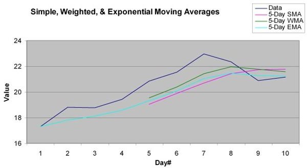
Remember to ignore the EMA data from Day1 through Day4. Notice that all 3 moving average lines have the same basic shape. That’s because they each show the overall trend, which is rising as the data values increase and then decline as the data values are less than the moving average value. The value in each of the different average computation methods is how quickly the average reacts to the data and how each individual data value affects the average. The EMA rises more quickly than the SMA but not as quickly as the WMA. This is because the WMA “front weights” the data, and for Day5, Day6, and Day7 the data is rising. Since the EMA also contains the data from Day1 through Day4, those lesser values cause the EMA to rise more slowly. Also notice that for Day8 through Day10, the EMA declines just as does the WMA, but at a slightly slower rate, again due to the effect from al previous data values that contribute to each day’s EMA value.
Conclusion
We now see how SMA, WMA, and EMA each reflect the trend of the data being averaged. We can now use these different moving average methods to determine short- and long-term trends in stocks, indices, mutual funds, currencies, or any other vehicle that trades on the world financial markets. These moving averages are combined to form composite indicators, or are used individually or in comparison to define trends.
Now that we’ve got these tools, we’ll venture into some technical analysis indicators to see what such indicators can tell us about past actions and likely upcoming actions.