Need help navigating some of the new features found in Excel 2007? This guide will walk you through the basics as well as through some of the more advanced functionalities.
What’s New in Excel 2007
What’s new in Excel 2007? Its number crunching, for starters. Excel 2007 gives you massively more rows and columns per worksheet, compared to previous Excel versions: 1,500 and 6,300 percent more rows and columns. Excel 2007 also sniffs out souped-up CPUs to more efficiently crunch those extra numbers.
The Ribbon
Excel 2007 has looks to match its muscles, including a new “uber-toolbar” called the Ribbon. The Ribbon was designed to enable fast access to the tools and functions you use most often.
A key benefit of the Ribbon is that it saves you from having to dig down into menus to access the tools you need. The odds are that, whichever tool you’re looking for, it will already be on the Ribbon, rather than buried in some place requiring a heap of keystrokes or mouse clicks to get to.
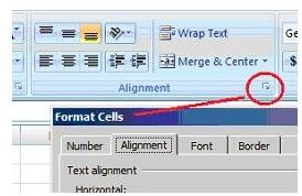
If you do need access to a lesser-used function, get it through the Dialog Box Launcher. That’s what the little arrow in the lower right corner of each command group is called.
_
One thing you can’t do in Excel 2007 that you could do (to excess) in prior versions of Excel is customize the toolbar, AKA the Ribbon. In prior versions of Excel, you could right click on a tool bar or menu, select Customize, and arrange your toolbars any way you wanted. However, with Office 2010, you will be able to customize the Ribbon .
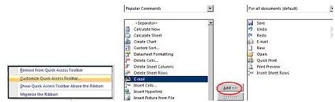
Excel 2007 replaces this functionality with a way you can customize the Quick Access Toolbar. Try this customization, which will place the icon for any tool you want on the Quick Access Toolbar:
- Right-click anywhere on the Quick Access Toolbar.
- Select “Customize Quick Access Toolbar.”
- Choose an icon from the left panel and click the Add button to install it on the Quick Access Toolbar.
- Click OK.
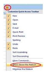
You can place a lot of icons on the Quick Access Toolbar this way, so don’t over mourn the loss of the old anything-goes toolbars. You can also move the Quick Access Toolbar itself: left-click on its arrow, then click Show Above/Below the Ribbon.
For a closer look at the Quick Access Toolbar, see Customizing and Adding Buttons to the Excel 2007 Ribbon .
Keyboard Shortcuts

If you’re still not sold on the Quick Access Toolbar, try this: load up the Quick Access Toolbar with eight or nine icons, then return to the worksheet. Press and release the Alt key and notice the numbers that appear on the Quick Access Toolbar icons. Those numbers represent keyboard shortcuts. Press Alt and any of those numbers to run the corresponding icon’s tool.
Learn more Excel shortcuts from Microsoft Excel CheatSheet for Beginners .
Improved Sorting and Filtering
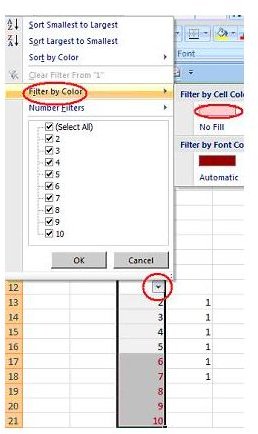
Excel 2007 adds the ability to sort and filter by color instead of just by data. Try this example that illustrates color filtering:
- On any worksheet, create a column of numbers from 1 to 10. (Tip: enter just the 1 and 2, select their cells; hover the pointer over the lower right corner until the pointer becomes a cross, then drag down until you have 10 numbers.)
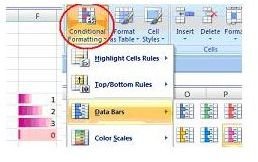
- Add conditional formatting to highlight the top 50 percent of the list: select the list, then choose Conditional Formatting>Top/Bottom Rules>Above Average. Click OK.
- Filter the list by color. With the list still selected, select Sort&Filter>Filter. Click the list’s filter arrow, choose Filter by Color, Filter by Cell Color, and choose the colored rectangle. Excel filters the list to show just the colored cells (the top 50 percent).
Read more about Excel’s Filter function from Microsoft Excel Help: Quickly Filter A List .
Calculated Columns
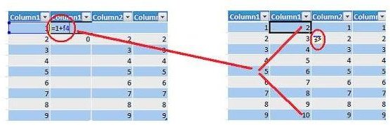
Excel 2007’s Calculated Columns feature makes entering formulas in tables much easier than in previous versions. Previously, if you had a table of data that needed a formula calculated for each row, you would have had to manually click and drag the top cell containing the initial formula. Now, you need only enter the formula in the first row; Excel will fill in the remaining ones. Try this example to watch calculated columns in action:
- Fill a worksheet range of at least three rows and three columns with numbers.
- Select Insert>Table, then click OK to create a table.
- Choose a single, non-header cell in the table.
- Choose Insert>Insert Table Columns to the Left.
- At the top non-header cell of the new, blank column, enter any formula (e.g. “=1+b2”).
- Notice that the Excel fills the complete column with your formula.
Easier Pivot Tables with Microsoft Excel 2007
Excel 2007 makes pivot table creation much easier than in prior versions: Excel visually guides you through each step of the table’s creation, and follows up by enabling easy rearrangement of the table’s fields.
Create a small pivot table to prove for yourself that the new interface is easier:
- Create a table like the following:
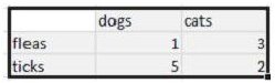
- Select the range, then select Insert>PivotTable.
- Press OK to accept the default configuration.
- In the Pivot Table Field List, click the Dogs and Cats checkboxes.
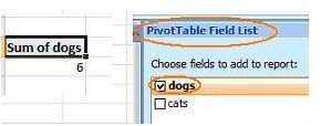
Notice that Excel automatically summarizes the flea and tick data. But, through the PivotTable Field List pane, it also lets you reconfigure the table easily, by enabling drag and drop of the table fields, and other tasks. This pane disappears when you click away from your pivot table, but will reappear when you click anywhere inside the table.
Read more about using Excel’s Pivot Tables from Making and Using Pivot Tables in Excel .
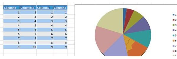
Cooler Looking Charts
Making hip-looking charts is easier in Excel 2007 compared to prior versions. Using Insert>Chart, you can create the ho-hum 3D pie chart on the right of the following figure from the data on the left:
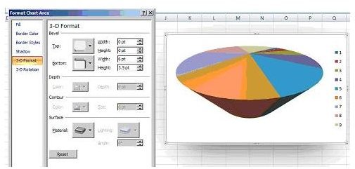
Then you can supercharge that chart by right-clicking it, choosing “3-D rotation,” then tinkering with the X, Y, and Z values, followed by the 3-D format options.
Create templates from your Excel charts by reading How to Create a Chart Template in Excel 2007
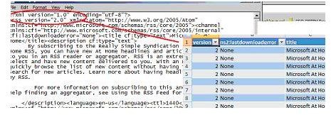
Excel 2007 Loads XML Files
With Excel 2007, you can now load the essential XML file format. Load these files as you would any other file type. Excel will give you the option to do a straight read of the file as table data, or as a tree of elements. If you’re not sure which you need, chances are it’s the table data, which is the default option.
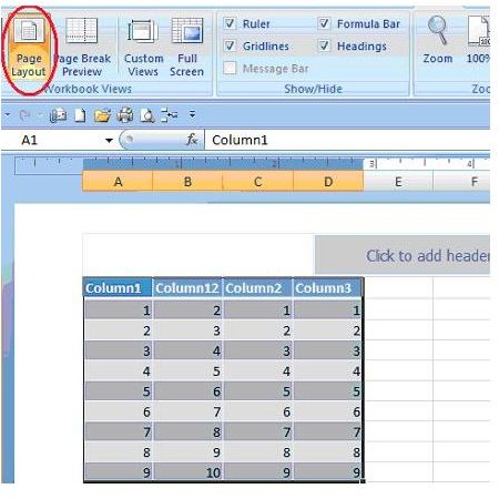
Page Layout View
Excel now offers a page layout view to give you a clear idea of how your worksheets will appear when printed. Access Page Layout through View>Page Layout.
Excel’s developers could likely have produced a worthy product if they’d simply added more functionality–reading XML files, or enabling conditional formatting, for example. But, by improving Excel’s user interface, they’ve made a product that’s also agreeable to look at and use.
References:
Microsoft Excel Help


