Making and Using Pivot Tables in Excel

Making a Pivot Table

Excel pivot tables are interactive reports. They condense and analyze data, which can be from a single Excel worksheet, multiple worksheets, or even external sources.

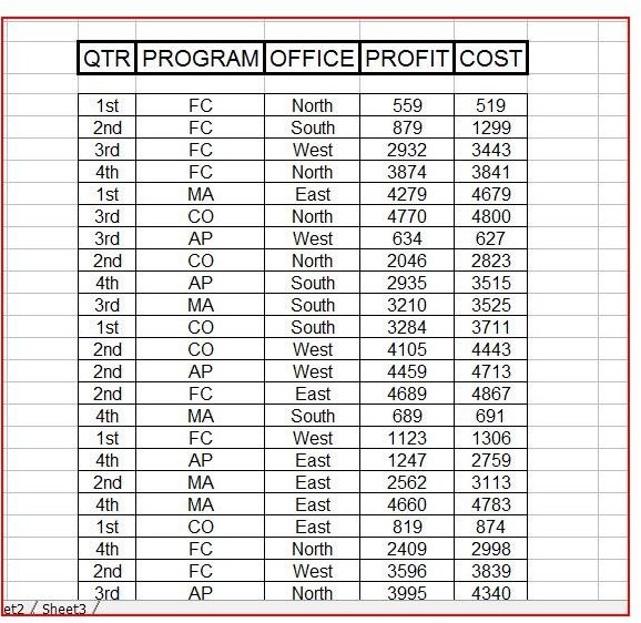
To begin, you will need some raw data to “pivot.” You will need at least two measures of data to work with, and with pivot tables the more data the merrier. Our example lists profits and costs for different departments in different office during different quarters.

If you are using Excel 2007, you will need to add the Pivot Table Wizard to your QAT (Quick Access Toolbar) for these steps to work correctly. To add the Pivot Table Wizard to the QAT, click the drop down arrow on the QAT. Select “PivotTable and PivotChart Wizard” from the list of commands, and click Add to add it to the QAT.

Place the cursor anywhere in the data you want to use in the pivot table. Click the Pivot Table Wizard from the QAT in Excel 2007, or go to the Data menu and select Pivot Table and Pivot Chart Report in Excel 2003 or earlier. The Pivot Table Wizard will open.

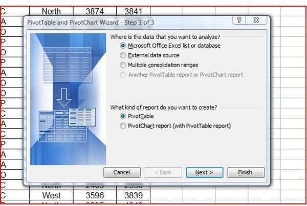
Select the location of the data you want to use. In our example, the data is in an Excel spreadsheet, so we will select Microsoft Excel List or Database. Select Pivot Table under What Kind of Report Do You Want to Create? Click Next.

Step 2 of the Pivot Table Wizard will request the location of the data you want to use. In our example, Excel “guesses” that we want to use the entire table. Since this is correct, we will click next. If it was not correct, you would either select the correct range of cells or click Browse to find the data.

Step 3 of the Wizard allows you to choose a location for your Excel pivot tables. Choose from the existing worksheet or a new one and click Finish. The Pivot Table Field List window will open.

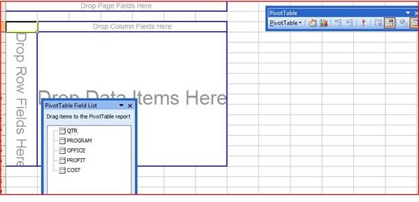
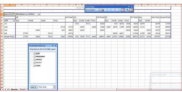
Drag and drop fields that you want to display in columns or fields. Click on the example to see how dragging and dropping the fields creates an instant report based on the data chosen.

To make your pivot table report look cleaner and more professional, use the AutoFormat feature. From the Pivot Table toolbar, select Format Report. Select an Excel pivot tables style and apply it to the report.

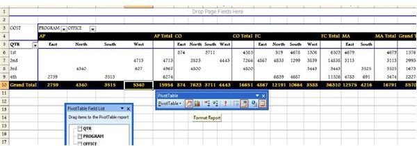
The last step is where “pivoting” comes into play. You can easily alter the resulting report by dragging and dropping fields into and out of the pivot table. The more data fields you have, the more report possibilities there are. And the more you work with Excel pivot tables, the more potential you will find for them, such as grouping data by weeks or present data in order by revenue.