Excel Help: Add A Customer Number To Each Detail Record, By Mr. Excel
Strategy:
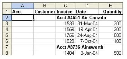
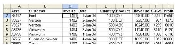
- Insert new columns A and B. Add headings of Acct and Customer, as shown in Fig. 836.
Here is the basic logic of what Excel want to do in plain language: Look at the first four characters of column C. If they are equal to “Acct”, then this row has customer information. Take data from that cell and move it to column A. Otherwise, if the first four characters are anything other than “Acct”, use the same account information from the previous row’s column A.
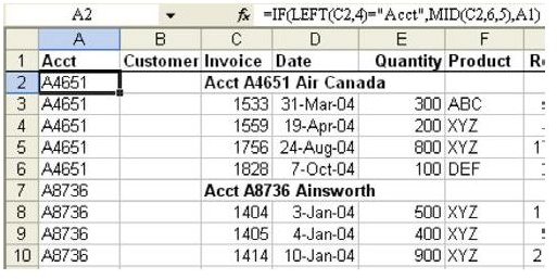
The formula to do this for cell A2 is as follows: =IF(LEFT(C2,4)=“Acct”,MID(C2,6,5),A1)
- Enter this formula into cell A2 and copy it down through column A.
As shown in Fig. 837, as you copy this formula down, it does the job. In cell A2, the IF condition is true and data is extracted from C2. In cell A3, the condition is not true, so the value from A2 is used. Down in cell A7, a new customer number is found so the data from C7 is used in A7. Cells A8 through A59 get the customer number from A7.
Similar logic is needed in column B. In this case, though, you need to grab the customer name. You know that the word “Acct” and the space that follows it take up five characters. You know that your account number is another five characters and then there is a space before the customer name. Thus, you want to ignore the first 11 characters of cell C2.
You can use a formula of =MID(C2,12,50) to skip the first 11 characters and return the next 50 characters of the customer name. However, this formula will add spaces to the end of the customer name to ensure that you have 50 characters in the result. You really don’t want all of those trailing spaces. The =TRIM() function will remove leading and trailing spaces from text.
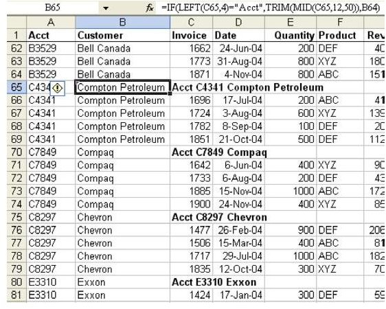
Use =TRIM(MID(C2,12,50)) as the formula to extract a customer name. Use this formula as the True portion of the IF function. As shown in Fig. 838, the formula in B2, copied down through column B, is as follows:
=IF(LEFT(C2,4)=“Acct”,TRIM(MID(C2,12,50)),B1)
- Enter this formula into cell B2 and copy it down through column B.
You have now successfully filled in account and customer. You need to change these formulas to values.
- Highlight columns A and B. Hit Ctrl+C to copy. Choose Edit – Paste Special – Values to convert the formulas to values.
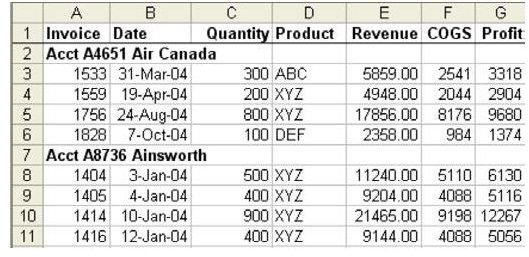
The last task is to remove all of the customer heading rows. As you look for a method to isolate the heading rows, you will notice that heading rows are the only rows with blank cells in column D. You can move the blanks to the end of a dataset by sorting the data by column D.
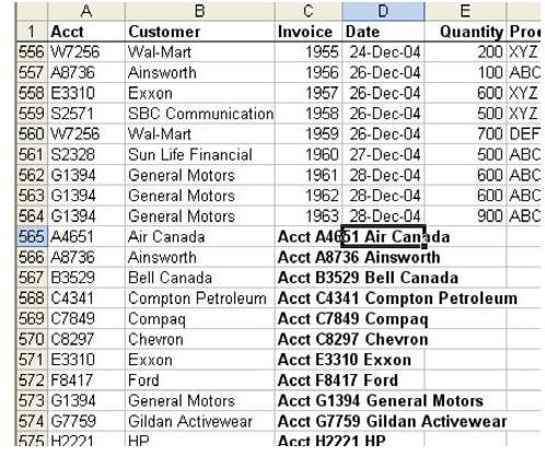
- Select the heading in D1. Hit the AZ sort button to sort ascending by Date. Any rows without a value in column D will automatically sort to the bottom of the dataset, as shown in Fig. 839.
- From D1, press the End key and then the Down Arrow key twice. The cell pointer will be located on the first customer heading. Delete all of the rows below row 564.
**
Result:
You have a clean dataset with customer information on every row, as shown in Fig. 840. You can sort this data and otherwise use it for data analysis.
Summary:
A couple of formulas with IF functions help to snap this data into shape.
Commands Discussed:
=IF(); =LEFT(); =MID()
**
Images